Improving quantile-respectful density estimation for discrete distributions using jittering
In my previous posts, I already discussed the problem that arises when we try to build kernel density estimation (KDE) for samples with ties. We may get such samples in real life from discrete or mixed discrete/continuous distributions. Even if the original distribution is continuous, we may observe artificial sample discretization due to the limited resolution of the measuring tool. Such discretization may lead to inaccurate density plots due to undersmoothing. The problem can be resolved using a nice technique called jittering. I also discussed how to apply jittering to get a smoother version of KDE.
However, I’m not a huge fan of KDE because of two reasons. The first one is the problem of choosing a proper bandwidth value. With poorly chosen bandwidth, we can easily get oversmoothing or undersmoothing even without the discretization problem. The second one is an inconsistency between the KDE-based probability density function and evaluated sample quantiles. It could lead to inconsistent visualizations (e.g., KDE-based violin plots with non-KDE-based quantile values) or it could introduce problems for algorithms that require density function and quantile values at the same time. The inconsistency could be resolved using quantile-respectful density estimation (QRDE). This kind of estimation builds the density function which matches the evaluated sample quantiles. To get a smooth QRDE, we also need a smooth quantile estimator like the Harrell-Davis quantile estimator. The robustness and componential efficiency of this approach can be improved using the winsorized and trimmed modifications of the Harrell-Davis quantile estimator (which also have a decent statistical efficiency level).
Unfortunately, the straightforward QRDE calculation is not always applicable for samples with ties because it’s impossible to build an “honest” density function for discrete distributions without using the Dirac delta function. This is a severe problem for QRDE-based algorithms like the lowland multimodality detection algorithm. In this post, I will show how jittering could help to solve this problem and get a smooth QRDE on samples with ties.
Continuous distribution
First of all, let’s briefly discuss the connection between the quantile function, the cumulative distribution function (CDF), and the probability density function (PDF) for continuous distributions. As a continuous distribution example, we take the Gumbel distribution.
Here is the Gumbel distribution quantile function $Q_{\textrm{Gum}}(p)$:
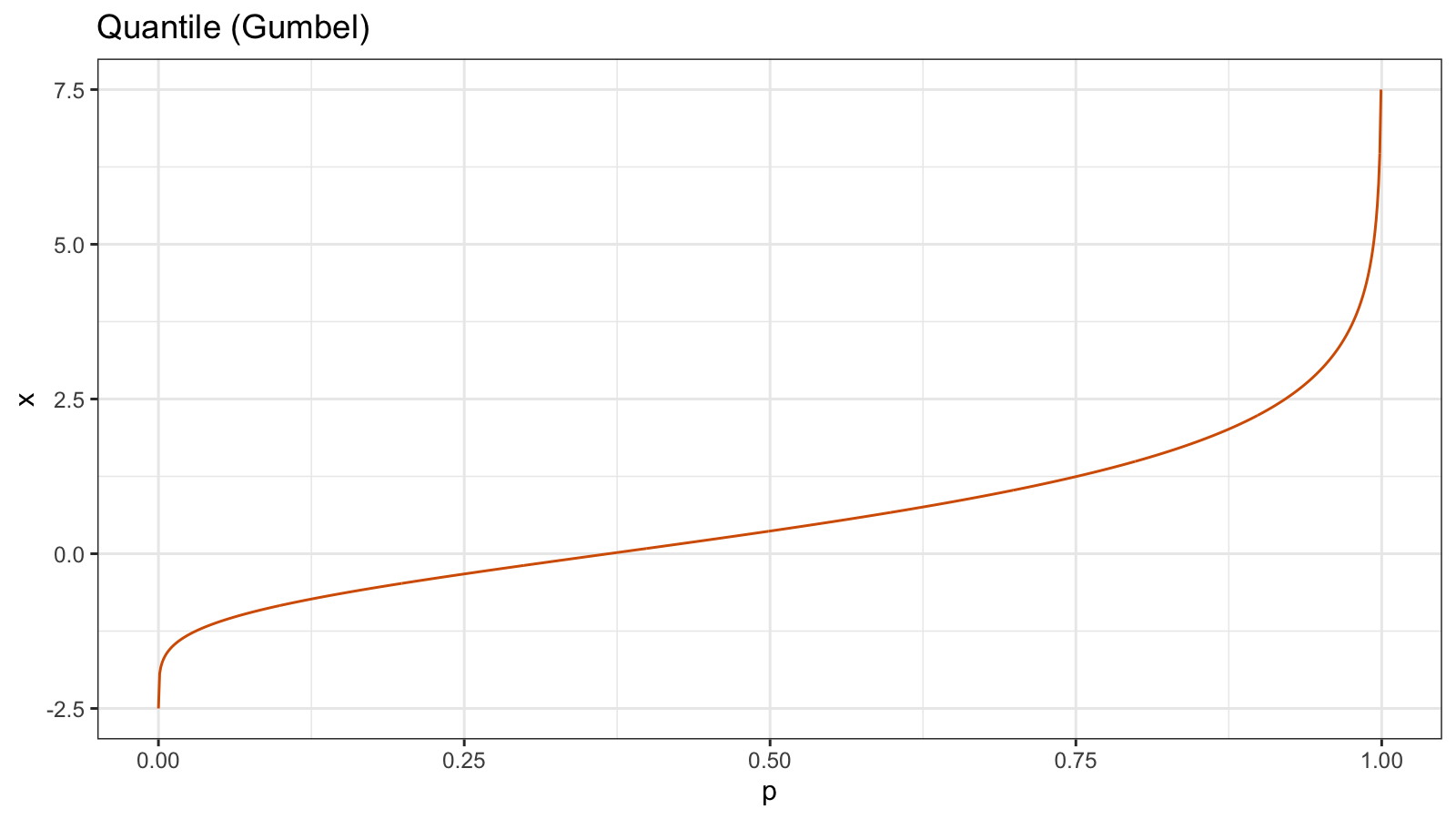
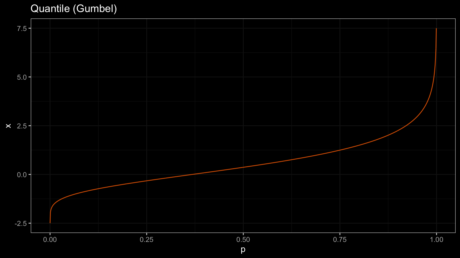
For the Gumbel distribution, all the quantile values are different. For any $p_1 < p_2$, we can say that $Q_{\textrm{Gum}}(p_1) < Q_{\textrm{Gum}}(p_2)$. It means that the quantile function $Q_{\textrm{Gum}}(p)$ is strictly increasing (it doesn’t have any horizontal segments).
The CDF is an inversion of the quantile function. Here is the CDF of the Gumbel distribution $F_{\textrm{Gum}} = Q^{-1}_{\textrm{Gum}}$:

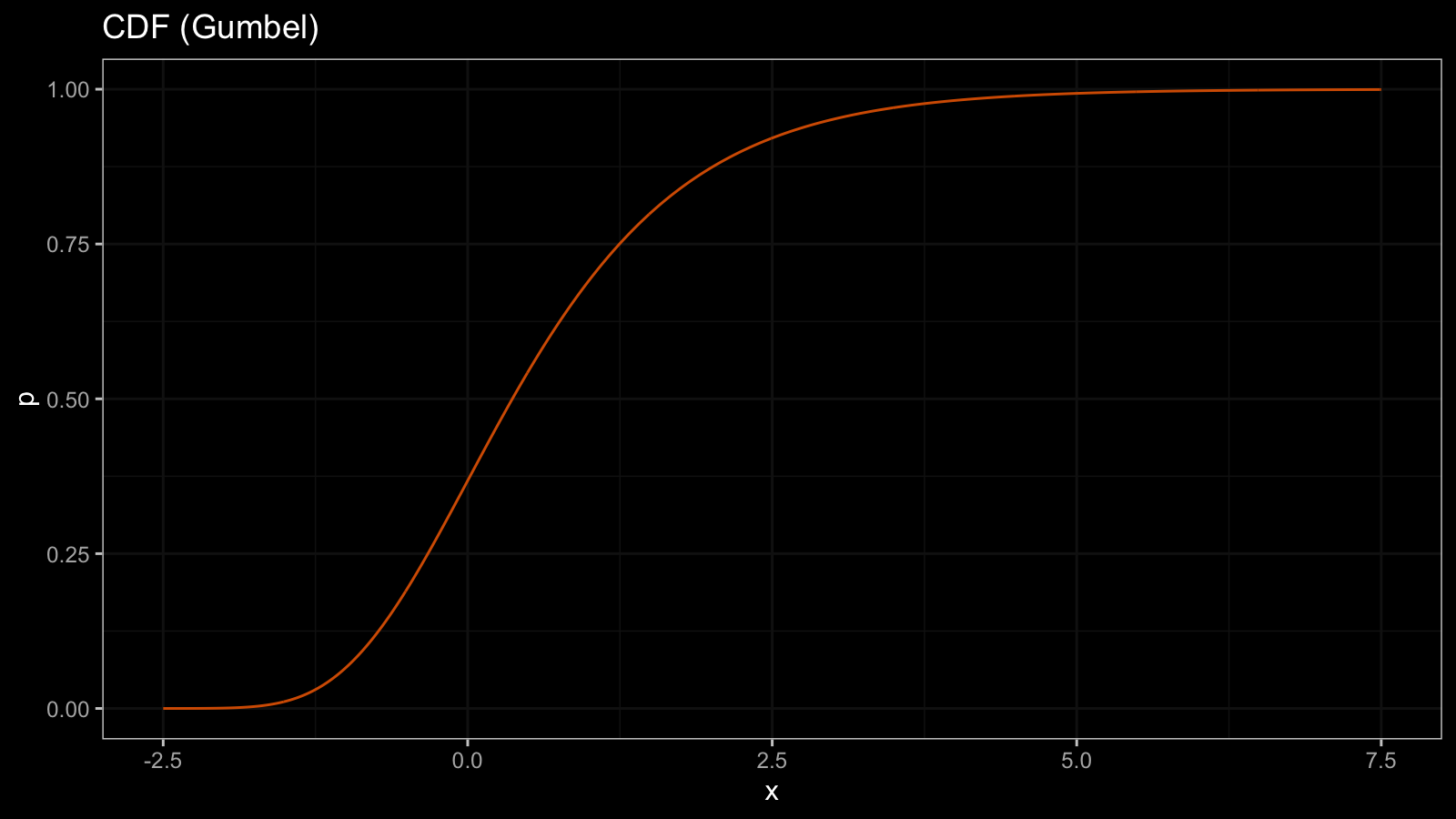
Since the quantile function doesn’t have horizontal segments, the CDF doesn’t have vertical segments. Thus, the CDF is also a continuous and strictly increasing function.
The PDF is the CDF derivative. Here is the PDF of the Gumbel distribution $f_{\textrm{Gum}} = F'_{\textrm{Gum}}$:

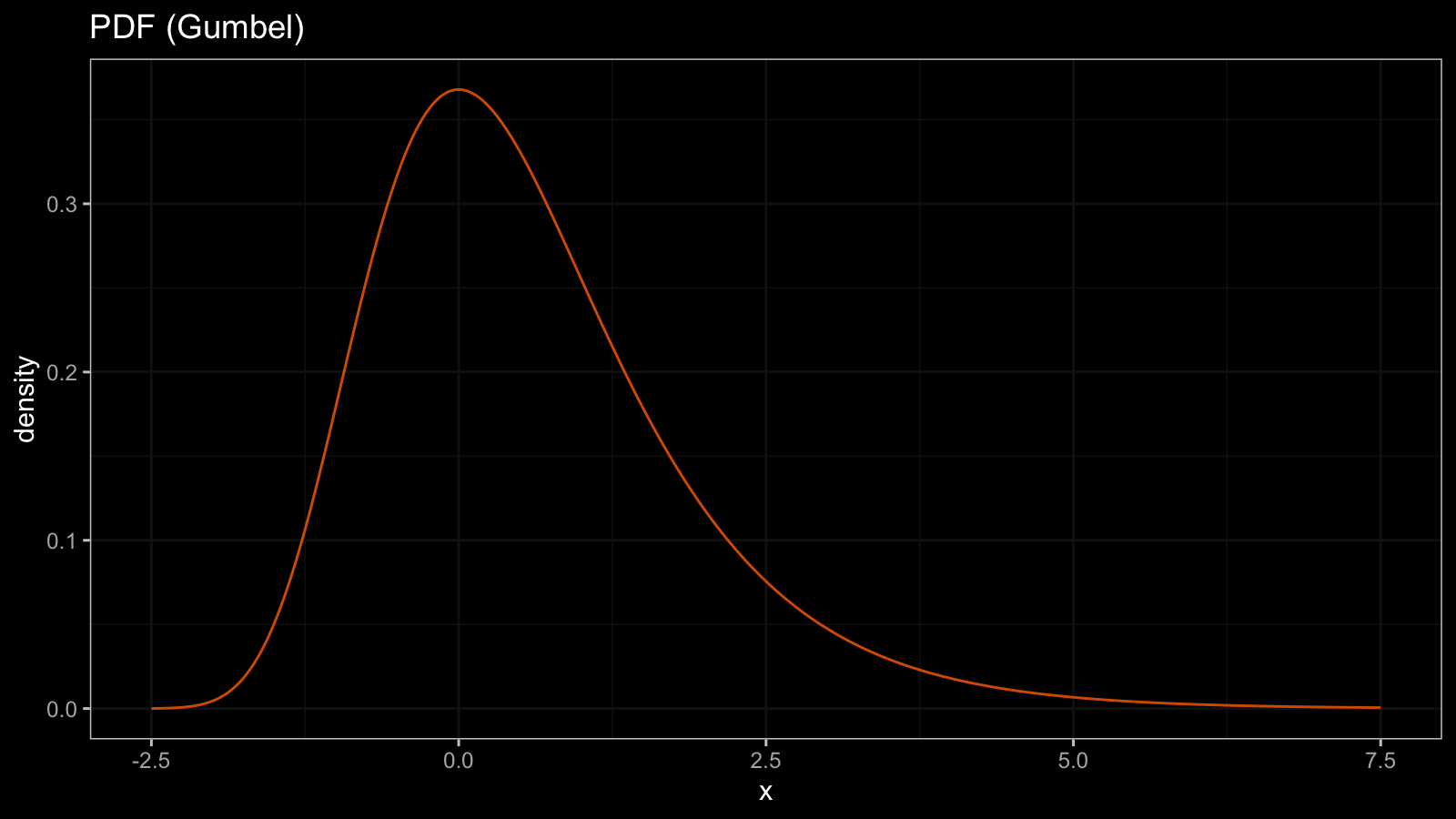
Since the CDF is continuous, the PDF is also a continuous function that has finite values at each point.
Discrete distribution
As a discrete distribution example, we take the Poisson distribution ($\lambda = 1$). Here is the corresponding quantile function $Q_{\textrm{Pois}}$:
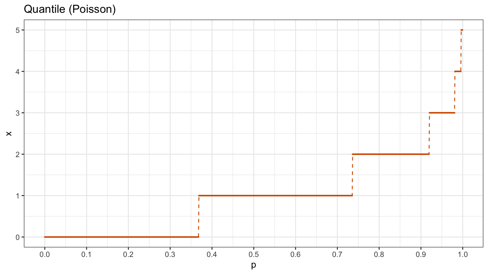
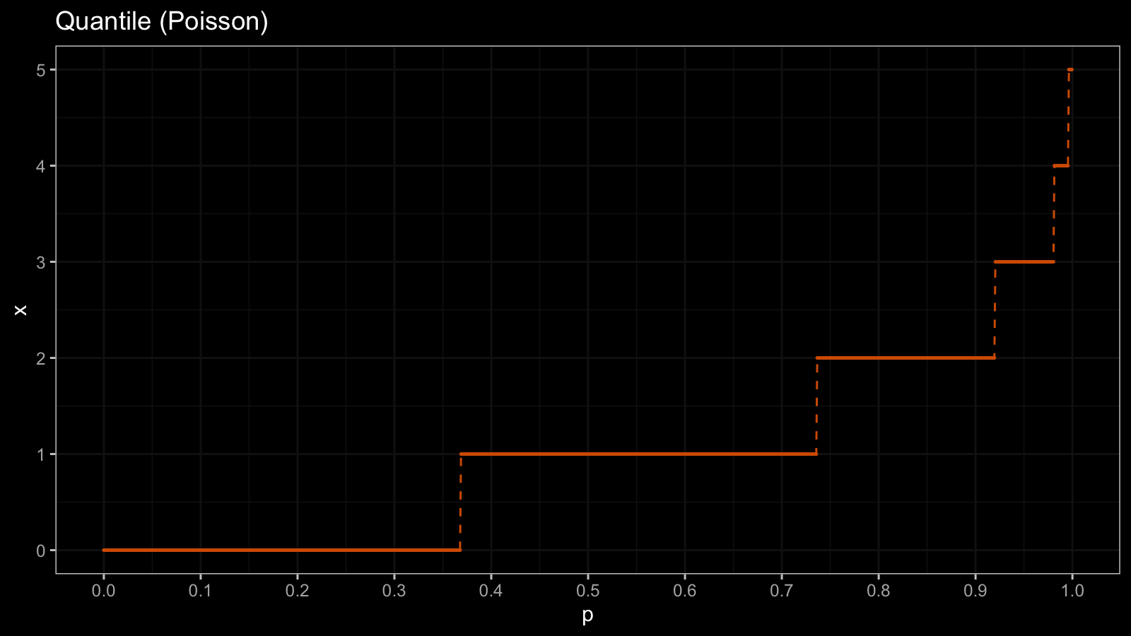
Since the Poisson distribution contains only integer numbers, the values of $Q_{\textrm{Pois}}$ are also integers. The quantile function consists of horizontal segments. Now let’s look at the CDF which is an inversion of the quantile function $F_{\textrm{Pois}} = Q^{-1}_{\textrm{Pois}}$:
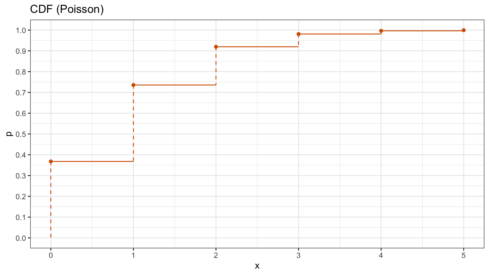
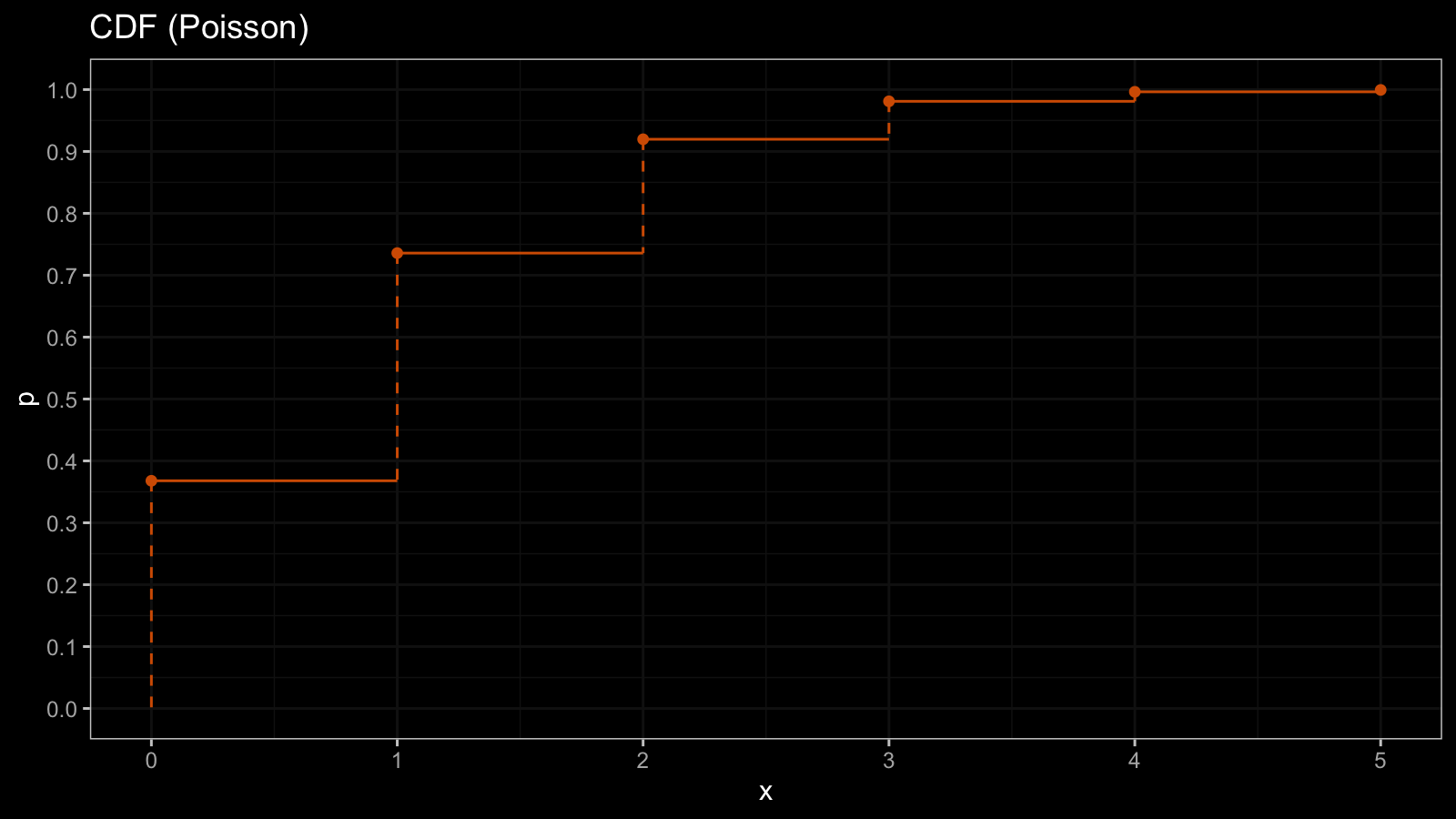
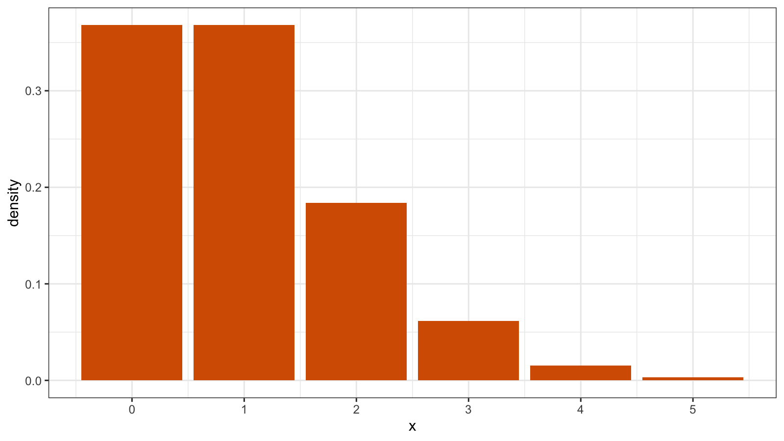
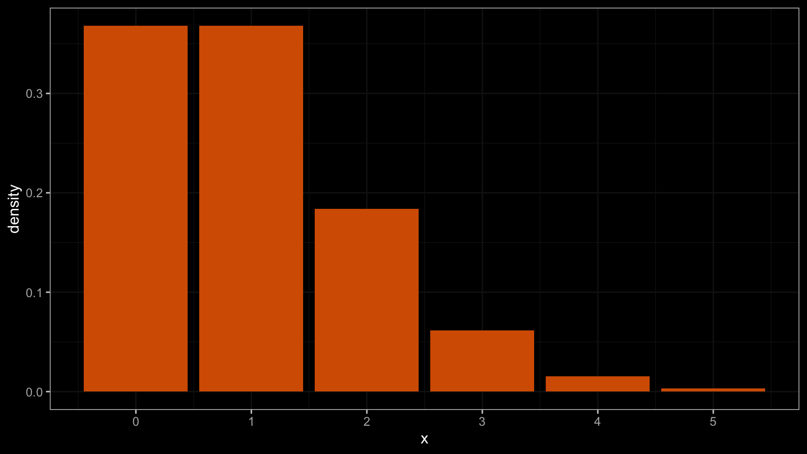
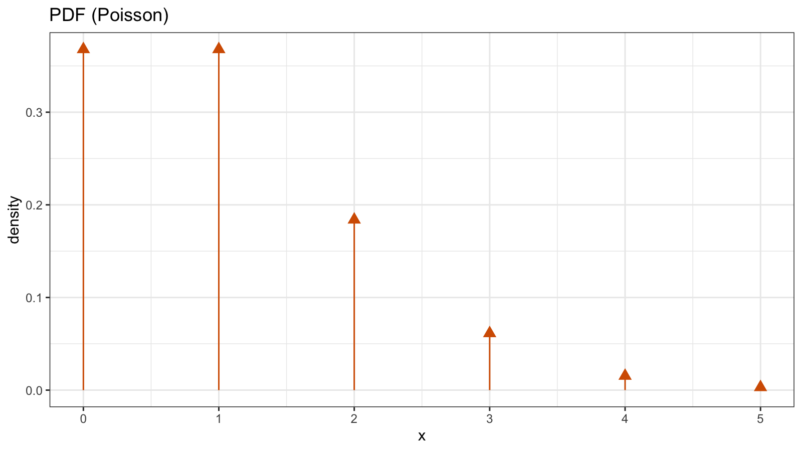
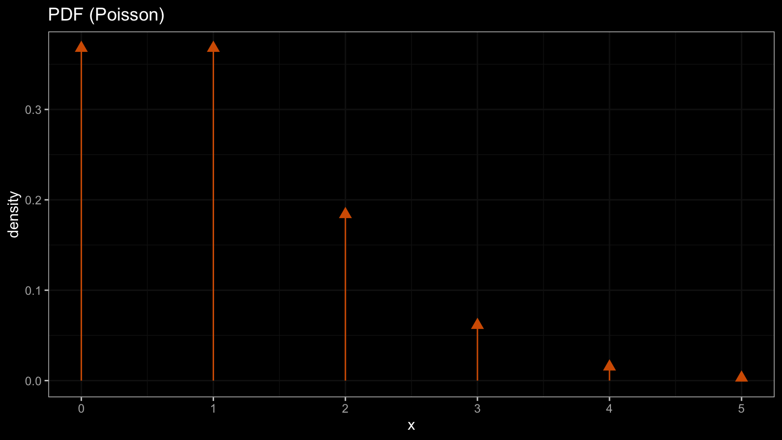
Since the quantile function has horizontal segments, the CDF is discontinuous at the integers. For discrete distributions, we typically use the probability mass function (PMF) instead of the PDF. Unlike the PDF, the PMF has a discrete argument, so it could be shown in the histogram form. Here is the PMF of the Poisson distribution:
If we really want to build the PDF, it’s possible with the help of the Dirac delta function:
Such PDF is not continuous.
QRDE
The detailed description and motivation of quantile-respectful density estimation (QRDE) can be found here. Let’s briefly recall the main idea of this approach. We are going to build a density estimation for a sample from an unknown distribution. This estimation should be consistent with the evaluated quantile values. To get a smooth estimation, we need a smooth quantile estimator like the Harrell-Davis quantile estimator (or its winsorized or trimmed modifications). Let $Q(p)$ be the target quantile estimator. Now we are going to estimate $k$-quantiles at the following positions:
$$ p_i = i / k, \quad i = 0, \ldots, k. $$For example, if $k = 100$ (we work with percentile), here are the $p_i$ values:
$$ p = \{ 0.00, 0.01, 0.02, \ldots, 0.99, 1.00 \}. $$The QRDE could be presented as a histogram. For each $i = 0, \ldots, k - 1$, we could introduce a histogram bar. The left ($x_l$) and the right ($x_r$) borders of the bar are defined as quantile values:
$$ x_l = Q(p_i), \quad x_r = Q(p_{i+1}). $$By definition, the total area of the density plot should equal $1.0$. If we split it into $k$ equal bars, the area of each bar should equal $1.0 / k$. Since we know the width and the area of each bar, it’s easy to calculate its height:
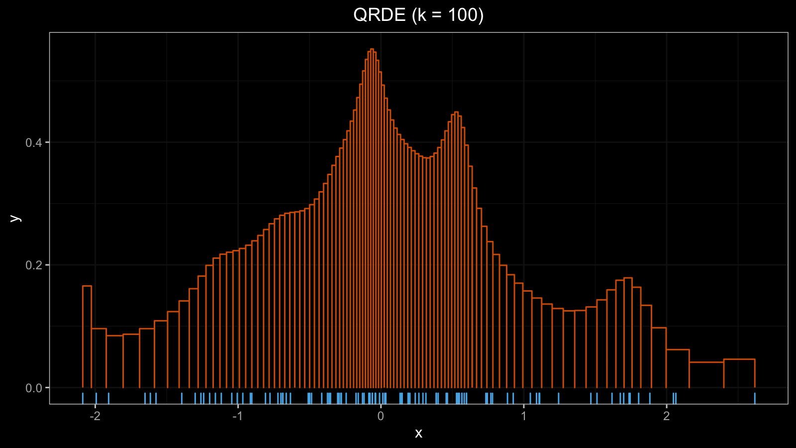
$$ h = \frac{1/k}{x_r - x_l} $$That’s all: now we know the borders and the height of each bar. Here is an example of the QRDE for a sample from the normal distribution (with a rug plot at the bottom):

Degenerate QRDE on discrete distribution
Let’s look one more time at the definition of the bar height:
$$ h = \frac{1/k}{x_r - x_l} = \frac{1/k}{Q(p_{i+1}) - Q(p_i)}. $$Thus, if $Q(p_i) = Q(p_{i+1})$, the histogram bar should be transformed to the Dirac delta function. In practice, if the given sample contains tied values, we may get a situation when $|Q(p_i) - Q(p_{i+1})|$ is extremely small, which leads to an extremely huge $h$ value. As a result, we get degenerated QRDE. Let’s check how it looks in real life.
Here is a sample from the Poisson distribution:
x1 = { 0, 2, 1, 0, 1, 1, 0, 0, 1, 1, 1, 1, 1, 1, 2 }
x1 gives us the following QRDE plot:
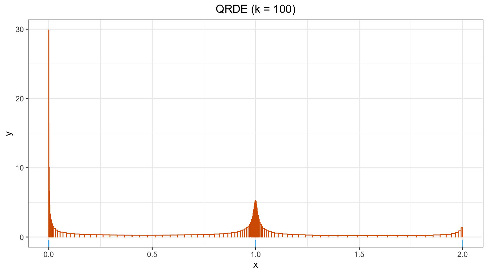
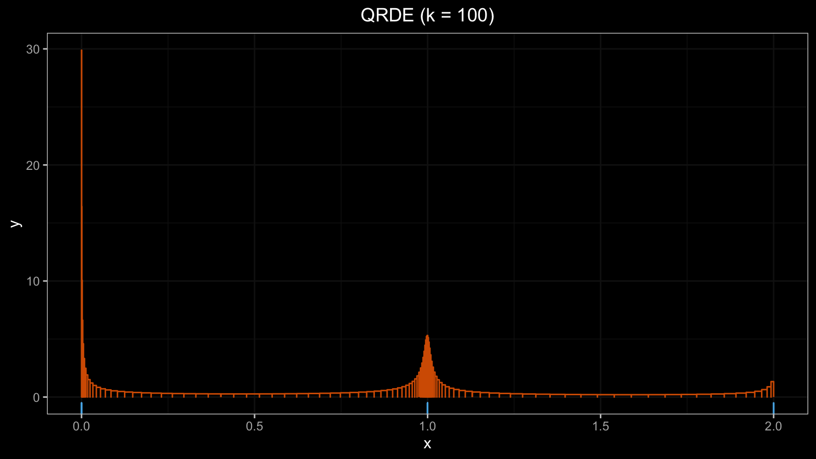
Because of the ties, we have a high peak around zero ($h \approx 30$).
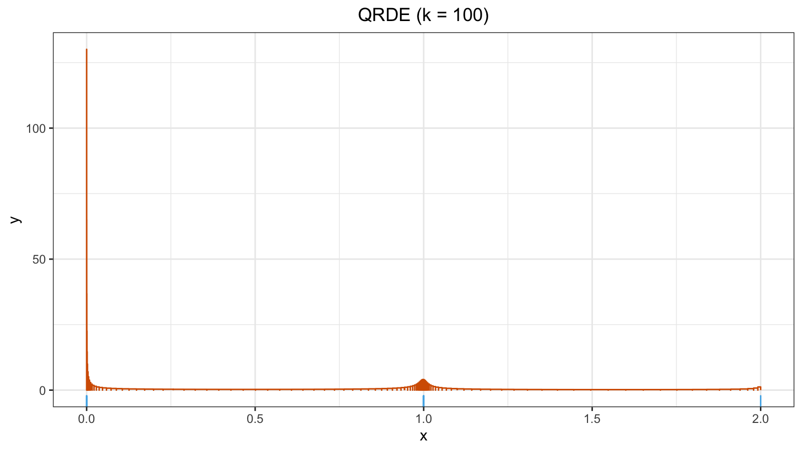
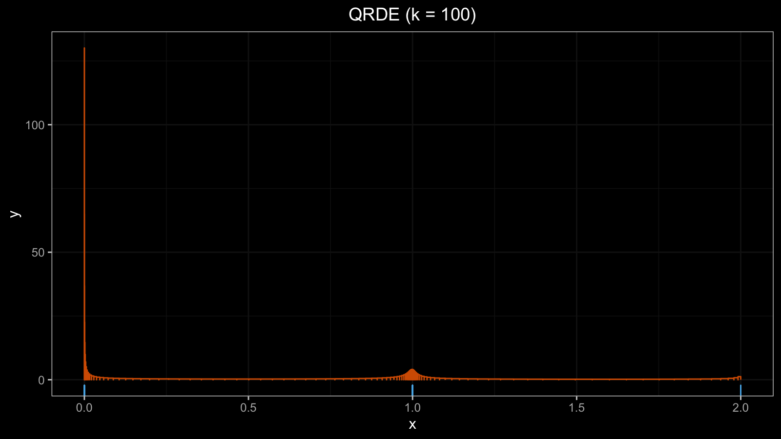
Now let’s add another zero value to x1:
x2 = {x1, 0} = { 0, 2, 1, 0, 1, 1, 0, 0, 1, 1, 1, 1, 1, 1, 2, 0 }
The situation became worse ($h \approx 130$):
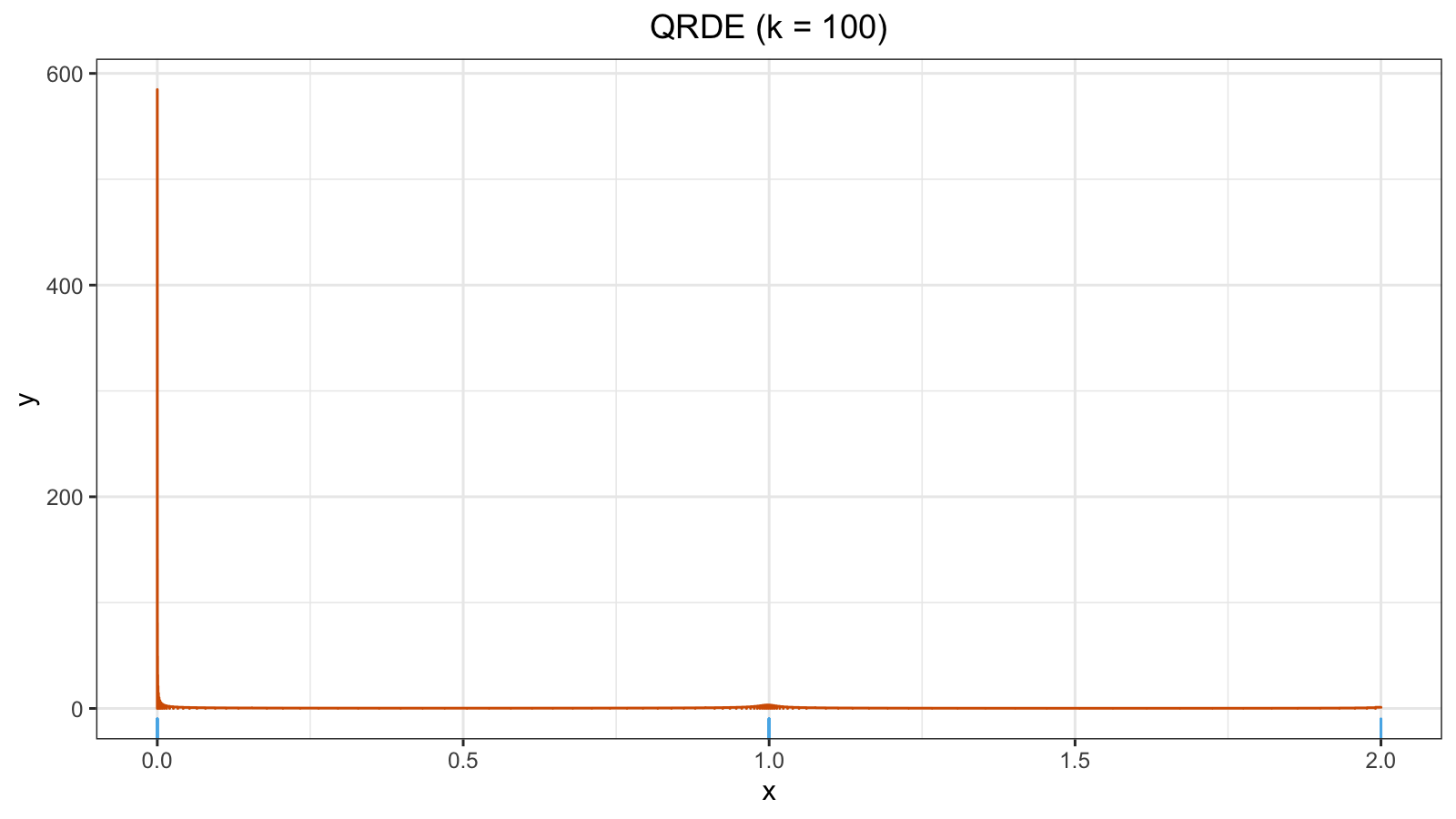
Let’s continue this procedure and add one more zero value:
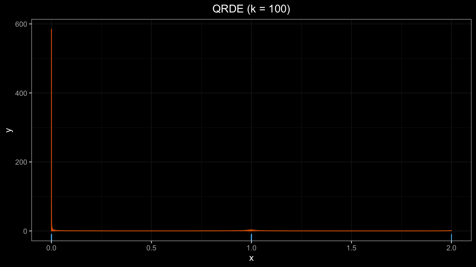
x3 = {x1, 0, 0 } = { 0, 2, 1, 0, 1, 1, 0, 0, 1, 1, 1, 1, 1, 1, 2, 0, 0 }
Now $h \approx 600$, the QRDE plot became useless:
Improving QRDE using jittering
To fix the problem, we can use the jittering technique based on the Beta function as described in the previous post. The suggested technique has the following advantages:
- It doesn’t involve randomization, so it produces the same result each time.
- It preserves the sample range: the minimum and the maximum value will not be corrupted.
- It ensures high density near the original values
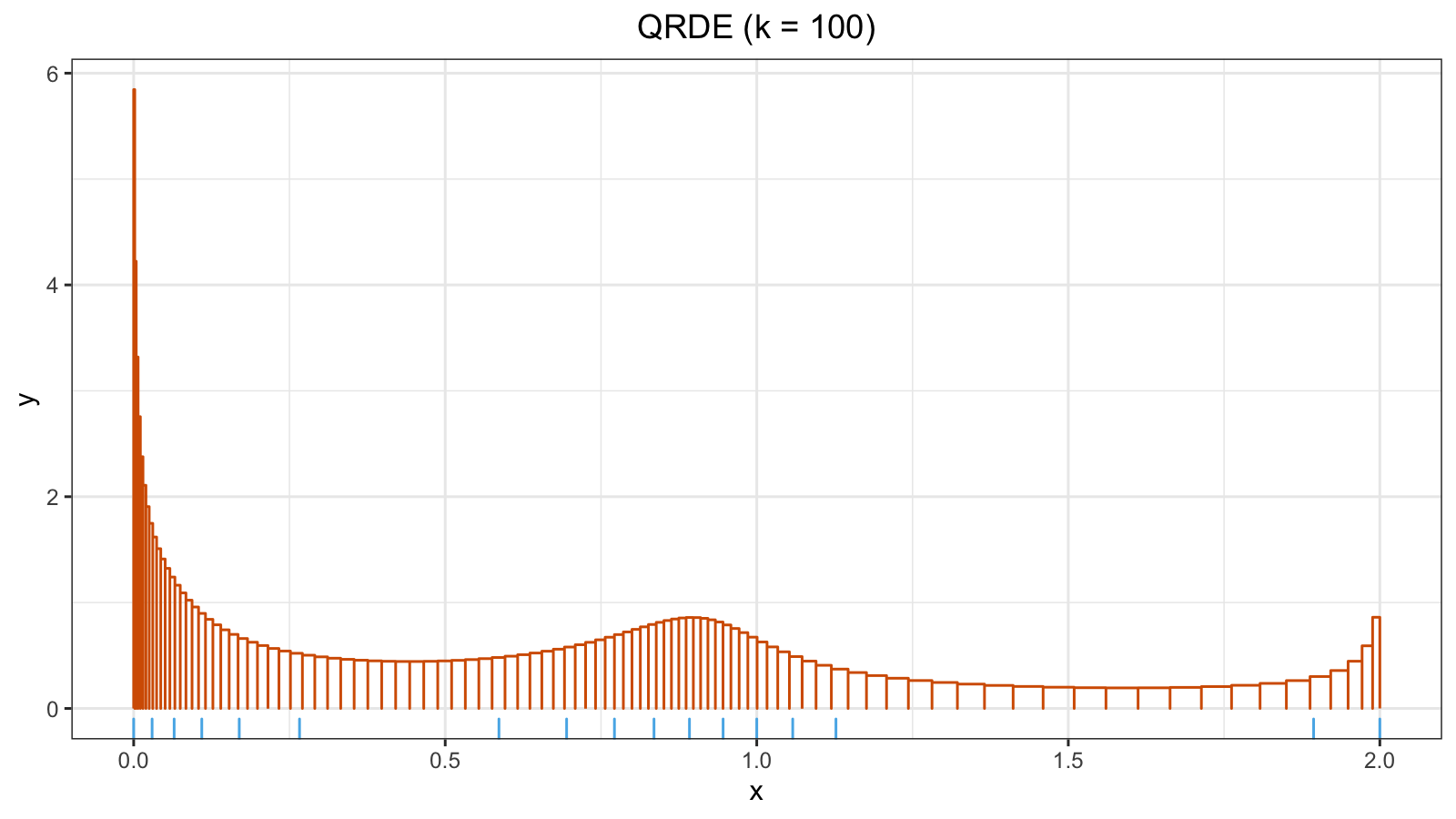
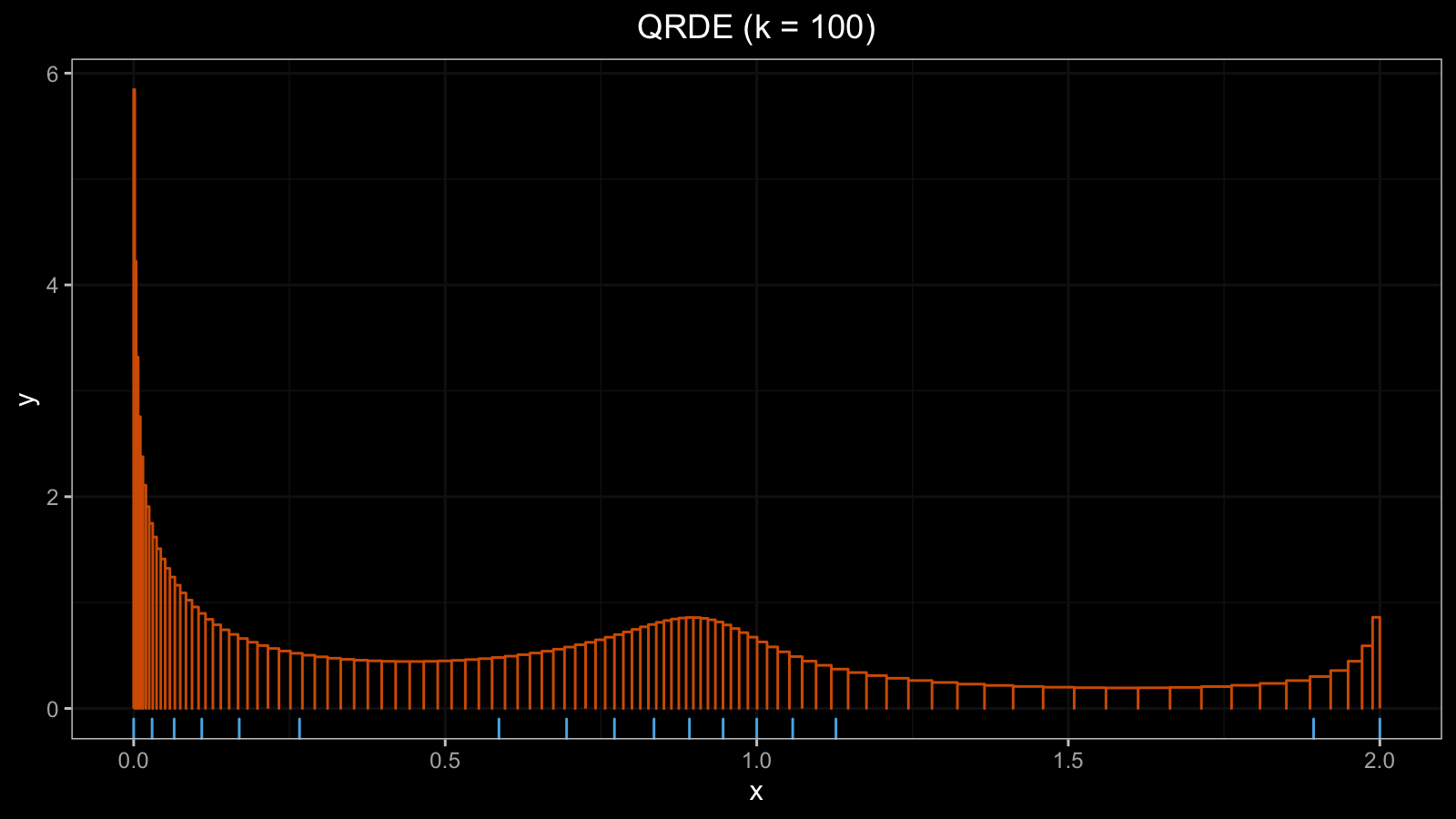
If we apply jittering (based on the Beta function) to x3, we get the following sample:
x4 = jittering(x3) = {
  0.00000000, 0.02957037, 0.06495575, 0.10929974,
  0.16944062, 0.26618052, 0.58622006, 0.69481940,
  0.77159043, 0.83508358, 0.89198685, 0.94597932,
  1.00000000, 1.05771731, 1.12709591, 1.89371011,
  2.00000000
}
This gives a reasonable QRDE plot: