Quantile-respectful density estimation based on the Harrell-Davis quantile estimator
The idea of this post was born when I was working on a presentation for my recent DotNext talk. It had a slide with a density plot like this:
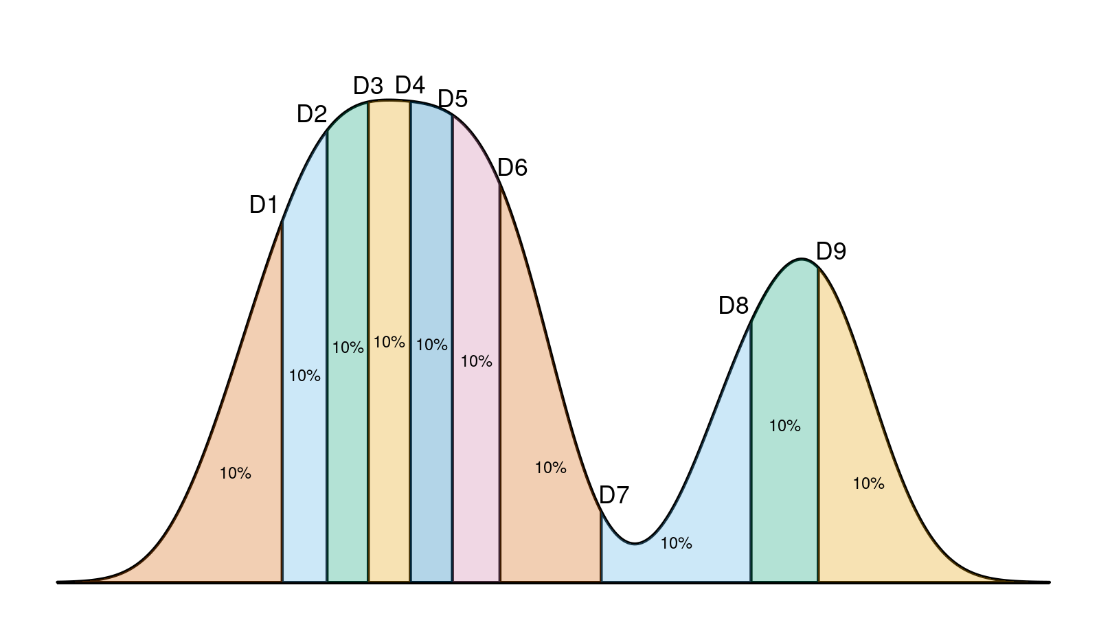
Here we can see a density plot based on a sample with highlighted decile locations that split the plot into 10 equal parts. Before the conference, I have been reviewed by @VladimirSitnikv. He raised a reasonable concern: it doesn’t look like all the density plot segments are equal and contain exactly 10% of the whole plot. And he was right!
However, I didn’t make any miscalculations. I generated a real sample with 61 elements. Next, I build a density plot with the kernel density estimation (KDE) using the Sheather & Jones method and the normal kernel. Next, I calculated decile values using the Harrell-Davis quantile estimator. Although both the density plot and the decile values are calculated correctly and consistent with the sample, they are not consistent with each other! Indeed, such a density plot is just an estimation of the underlying distribution. It has its own decile values, which are not equal to the sample decile values regardless of the used quantile estimator. This problem is common for different kinds of visualization that presents density and quantiles at the same time (e.g., violin plots)
It leads us to a question: how should we present the shape of our data together with quantile values without confusing inconsistency in the final image? Today I will present a good solution: we should use the quantile-respectful density estimation based on the Harrell-Davis quantile estimator! I know the title is a bit long, but it’s not so complicated as it sounds. In this post, I will show how to build such plots. Also I will compare them to the classic histograms and kernel density estimations. As a bonus, I will demonstrate how awesome these plots are for multimodality detection.
The problem
To understand the problem better, consider a sample with three elements: $x = \{ 3, 4, 7 \}$. Let’s build a probability density function (PDF) based on kernel density estimation using the Sheather & Jones method and the normal kernel. Let’s also calculate the median and the $95^{\textrm{th}}$ percentile using three different methods:
- Type 7 quantile estimator
It’s the most popular quantile estimator which is used by default in R, Julia, NumPy, Excel (PERCENTILE,PERCENTILE.INC), Python (inclusivemethod). We call it “Type 7” according to notation from Sample Quantiles in Statistical Packages
By Rob J Hyndman, Yanan Fan · 1996hyndman1996, where Rob J. Hyndman and Yanan Fan described nine quantile algorithms which are used in statistical computer packages. - The Harrell-Davis quantile estimator
A quantile estimator that is described in A new distribution-free quantile estimator
By Frank E Harrell, C E Davis · 1982harrell1982. It’s more efficient, and it provides more reliable estimations. - KDE-based quantile estimator
Quantile values that are obtained from the kernel density estimation instead of the original sample.
Here is the density plot with highlighted quantiles:


As you can see, all three quantile estimators produced different values. However, only the KDE-based quantile estimator is consistent with the density plot. For example, the KDE-based median estimation splits the density plot into two equal parts while two other estimators produce other ratios. The problem becomes more obvious if we look at the $95^{\textrm{th}}$ percentile. As we can see, the KDE-based value (7.73) is bigger than the maximum sample element $x_{\max} = 7$. It’s an expected situation: the kernel density estimation estimates the whole underlying distribution. If we use the normal kernel, some parts of the density plot will always be between $x_{\max}$ and positive infinity. It means that some of the high quantiles will always be bigger than $x_{\max}$. However, we can’t say the same about the Type 7 and Harrell-Davis quantile estimators. For a sample-based estimator, no quantile estimation can exceed $x_{\max}$.
Thus, it’s not a good idea to present sample-based quantile estimation with the kernel density estimation because they are not consistent with each other. To make it consistent, we have two possible solutions:
- Present KDE-based quantile values that are consistent with the existing density plot
- Present another density plot that is consistent with the existing quantile values
The first option may confuse people. Indeed, let’s say we want to present the $99.9^{\textrm{th}}$ percentile. In the case of the KDE-based quantiles, this value may be extremely high or even tend to infinity. Most people will expect to see a value based on the existing data rather than on the KDE.
Let’s try the second option, where we try to build a density plot using the estimated quantile values.
Quantile-respectful density estimation
Let’s introduce a new term: quantile-respectful density estimation1 (QRDE). It’s a density estimation that matches the given quantile values. Obviously, it highly depends on the used quantile estimator. In this section, we compare two different variations of QRDE that are based on the Type 7 quantile estimator (QRDE-T7) and on the HarrellDavis quantile estimator (QRDE-HD).
From the computational point of view, the easiest way to evaluate QRDE is to present it as a step function based on several quantile values. It’s convenient to consider the minimum and the maximum values as additional quantile values (although it’s not correct from the formal point of view). It’s also convenient to think about this step function as a density histogram. For each pair of consecutive quantiles values, we should draw a bin. The left and the right borders of the bin are equal to the quantile values. We want to make the QRDE consistent with the quantile values, so each bin’s area should be equal to $1 / p$ when we work with $p$-quantiles. Since we know the width and the area of each bin, it’s easy to calculate its height:
$$ h_i = \frac{\textrm{Area}_i}{\textrm{Width}_i} = \frac{1/p}{q_{i + 1} - q_i} = \frac{1}{p(q_{i + 1} - q_i)}. $$Now let’s look at some examples. For simplification, we start with deciles. They split our distribution into 10 equal sizes. Thus, we should get 10 bins, the area of each bin is 0.1. For the above sample $x = \{ 3, 4, 7 \}$, we have the following plots:


The Type 7 quantile estimator presents a nice visualization of this concept. The median of the sample (which equals 4 with the given estimator) splits the QRDE into two equal parts. Since this quantile estimator is based on linear interpolation, we have a flat area in each part.
The Harrell-Davis quantile estimator gives us more smoothness. At the start, you may be confused by the spikes at the ends of the plot. However, if you think about it a little bit, this phenomenon becomes pretty obvious and natural. Indeed, the sample’s corner elements are “magic” points, where a huge portion of density arises from nowhere. We have zero density on one side and a high positive density on another side. You may also observe such spikes with the KDE if you cut down parts before the minimum element and after the maximum element.
Now let’s increase the number of elements and consider a 500-element sample from the normal distribution:


We can recognize the bell-shape of the normal distribution, but it’s pretty rough. Also, we do not see a significant difference between the presented quantile estimators. The difference becomes more obvious if we reduce the quantization step value and switch to percentiles:


Now we can see that the Harrell-Davis gives us a smoother version of the QRDE. The Type7-based QRDE looks too spiky, which makes it not so useful. With a very small quantization step, it becomes completely useless because in most cases, we will observe only a few bins that have the maximum density:


Meanwhile, the Harrell-Davis-based QRDE keeps its smooth form:


Of course, it’s not as smooth as the KDE. We have such a wobbly plot because it describes our real data instead of oversmoothed estimation of the underlying distribution. If we don’t know the actual distribution and we want to just explore the data in the collected sample, the Harrell-Davis-based QRDE is one of the best ways to do it.
The most important fact about this plot is that it’s consistent with the quantile values. The estimated value of median splits this plot into two equal parts, the estimated decile values split this plot into ten equal parts, and so on.
QRDE and multimodal distributions
The true power of the QRDE manifests itself when you start working with multimodal distributions. Let’s check out some advantages of the QRDE against classic histograms and the KDE.
It highlights multimodality without parameter tuning.


Here we have a distribution with four modes (a combination of $\mathcal{N}(0, 4)$, $\mathcal{N}(0, 8)$, $\mathcal{N}(0, 12)$, $\mathcal{N}(0, 16)$; 30 elements from each). For the classic histogram, we should choose the offset and the bandwidth, which may be a problem. For KDE, we should choose the bandwidth and the kernel, which also may be problem. With Harrell-Davis-based QRDE, we don’t have any parameters to tune: the plot is uniquely defined, and it almost always presents what we want to see.
It highlights multimodality even if two modes are close to each other.


Here we have a bimodal distribution with background noise (1000 elements from $\mathcal{U}(0; 10)$, 100 elements from $\mathcal{N}(5, 0.1^2)$, 100 elements from $\mathcal{N}(5.5, 0.1^2)$). It’s always impossible to see signs of multimodality on the classic histograms or the KDE plots. Meanwhile, the Harrell-Davis-based QRDE solves highlights multimodality without any problems. When two modes are clearly expressed, we will always see it on such a plot regardless of the total range, the distance between modes, and the noise pattern.
It highlights multimodality even there are too many modes.


Here we have a multimodal distribution with 20 modes (a combination of $\mathcal{N}(4i, 1^2)$ for $i \in \{ 1..20\}$; 100 elements from each). It’s completely impossible to detect such multimodality using the KDE; these plots are too smooth for this problem. It’s also impossible to distinguish such a situation from regular noise using classic histograms (another example of the bandwidth problem). In contrast, the Harrell-Davis-based QRDE doesn’t have a limitation on the number of modes: it always able to detect all the modes while they are clearly expressed.
Conclusion
Currently, the QRDE-HD quantile estimator is my favorite way to present the collected sample’s raw shape. I want to highlight one more time two main advantages that I described in this post:
- Quantile-consistency
It’s safe to show quantile values on such a plot: it will always be consistent with the presented density. - Multimodality detection
It will not hide multimodality phenomena from you, which makes it a convenient tool to explore samples from non-parametric distributions. In future posts, I will present an algorithm that detects locations of all existing modes.
References
- [Hyndman1996]
Hyndman, R. J. and Fan, Y. 1996. Sample quantiles in statistical packages, American Statistician 50, 361–365.
https://doi.org/10.2307/2684934 - [Harrell1982]
Harrell, F.E. and Davis, C.E., 1982. A new distribution-free quantile estimator. Biometrika, 69(3), pp.635-640.
https://pdfs.semanticscholar.org/1a48/9bb74293753023c5bb6bff8e41e8fe68060f.pdf
In the first version of this post, I used term “empirical probability density function.” After some thoughts, I decided to rename it to “quantile-respectful density estimation.” The new term is not so confusing (the suggested function is significantly different from the empirical function) and it describes the underlying concept much better. Naming is hard. ↩︎