Quantile exponential smoothing
One of the popular problems in time series analysis is estimating the moving “average” value. Let’s define the “average” as a central tendency metric like the mean or the median. When we talk about the moving value, we assume that we are interested in the average value “at the end” of the time series instead of the average of all available observations.
One of the most straightforward approaches to estimate the moving average is the simple moving mean. Unfortunately, this approach is not robust: outliers can instantly spoil the evaluated mean value. As an alternative, we can consider simple moving median. I already discussed a few of such methods: the MP² quantile estimator and a moving quantile estimator based on partitioning heaps (a modification of the Hardle-Steiger method). When we talk about simple moving averages, we typically assume that we estimate the average value over the last $k$ observations ($k$ is the window size). This approach is also known as unweighted moving averages because all target observations have the same weight.
As an alternative to the simple moving average, we can also consider the weighted moving average. In this case, we assign a weight for each observation and aggregate the whole time series according to these weights. A famous example of such a weight function is exponential smoothing. And the simplest form of exponential smoothing is the exponentially weighted moving mean. This approach estimates the weighted moving mean using exponentially decreasing weights. Switching from the simple moving mean to the exponentially weighted moving mean provides some benefits in terms of smoothness and estimation efficiency.
Although exponential smoothing has advantages over the simple moving mean, it still estimates the mean value which is not robust. We can improve the robustness of this approach if we reuse the same idea for weighted moving quantiles. It’s possible because the quantiles also can be estimated for weighted samples. In one of my previous posts, I showed how to adapt the Hyndman-Fan Type 7 and Harrell-Davis quantile estimators to the weighted samples. In this post, I’m going to show how we can use this technique to estimate the weighted moving quantiles using exponentially decreasing weights.
Mean exponential smoothing
First of all, let’s recall the idea of the mean exponential smoothing. Let’s say we have a series $\{ x_1, x_2, \ldots \}$. The exponentially weighted moving mean can be defined as follows:
$$ \left\{ \begin{array}{l} s_1 = x_1,\\ s_i = \alpha x_i + (1 - \alpha)s_{i-1} \quad \textrm{for}\;\; i > 1 \end{array} \right. $$where $\alpha$ is the smoothing factor ($0 < \alpha < 1$). This recursive form allows calculation of the exponentially weighted moving mean using $O(1)$ complexity. However, this can be rewritten without recursion as a weighted sum of all observations $x_i$:
$$ s_n = \sum_{i=1}^n w_i x_i $$where
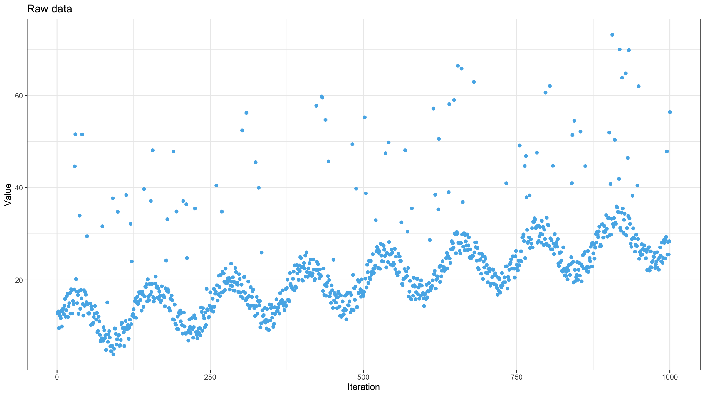
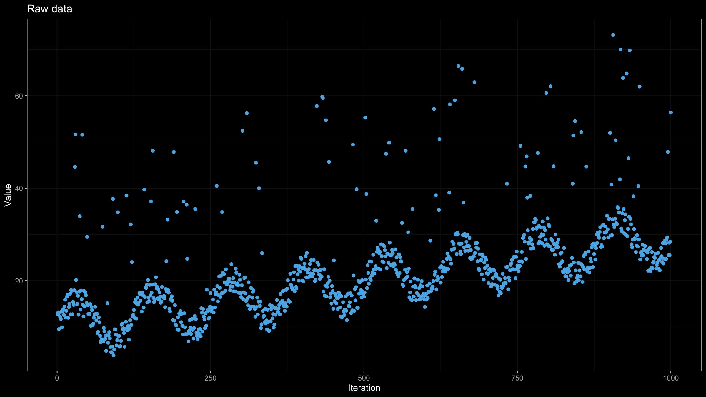
$$ \left\{ \begin{array}{l} w_1 = (1 - \alpha)^{(n-1)},\\ w_i = \alpha (1 - \alpha)^{n-i} \quad \textrm{for}\;\; i > 1 \end{array} \right. $$Now let’s try to test this approach. One of my favorite data sets for testing moving average estimators is a noisy, monotonically increasing sine wave pattern with high outliers. Here is how it looks like:
Now let’s calculate the exponentially weighted moving mean using $\alpha = 0.9$:
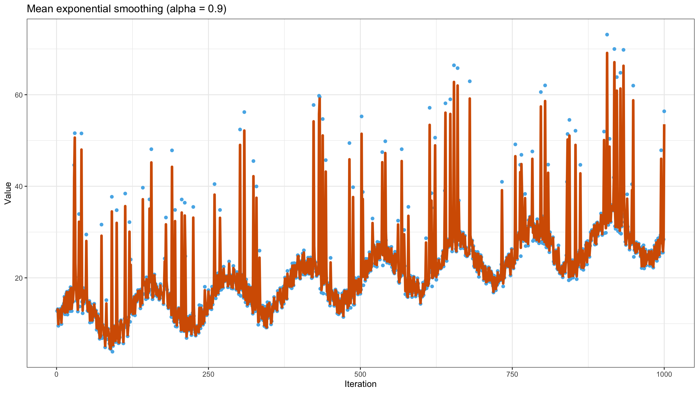
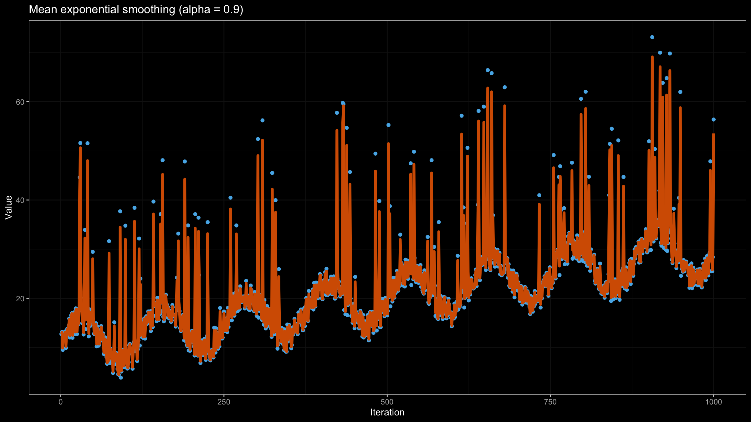
As we can see, exponential smoothing doesn’t help us to get a smooth line. The values of the moving mean are heavily affected by outliers. Let’s try to reduce the value of $\alpha$ to $0.5$:
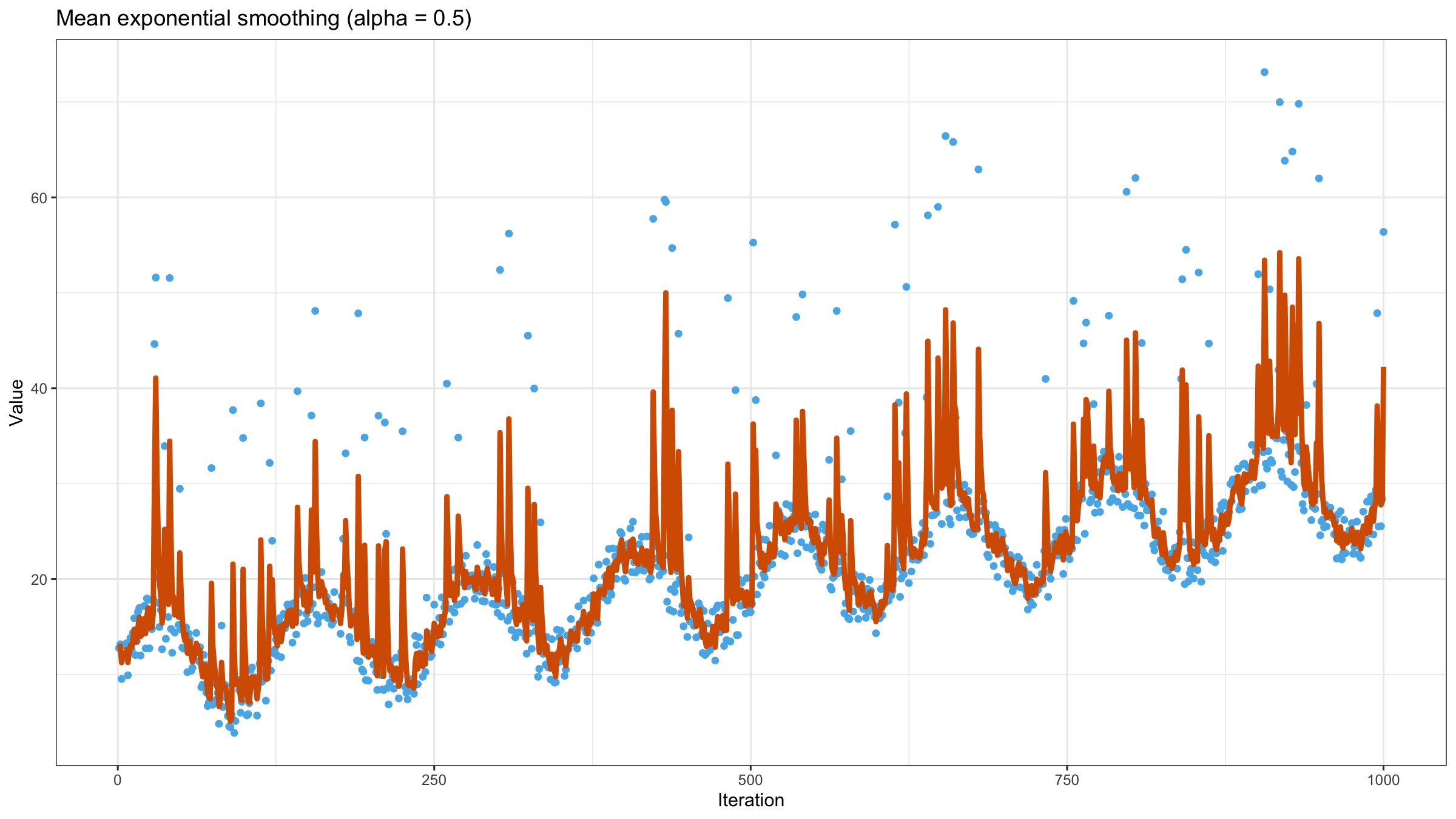
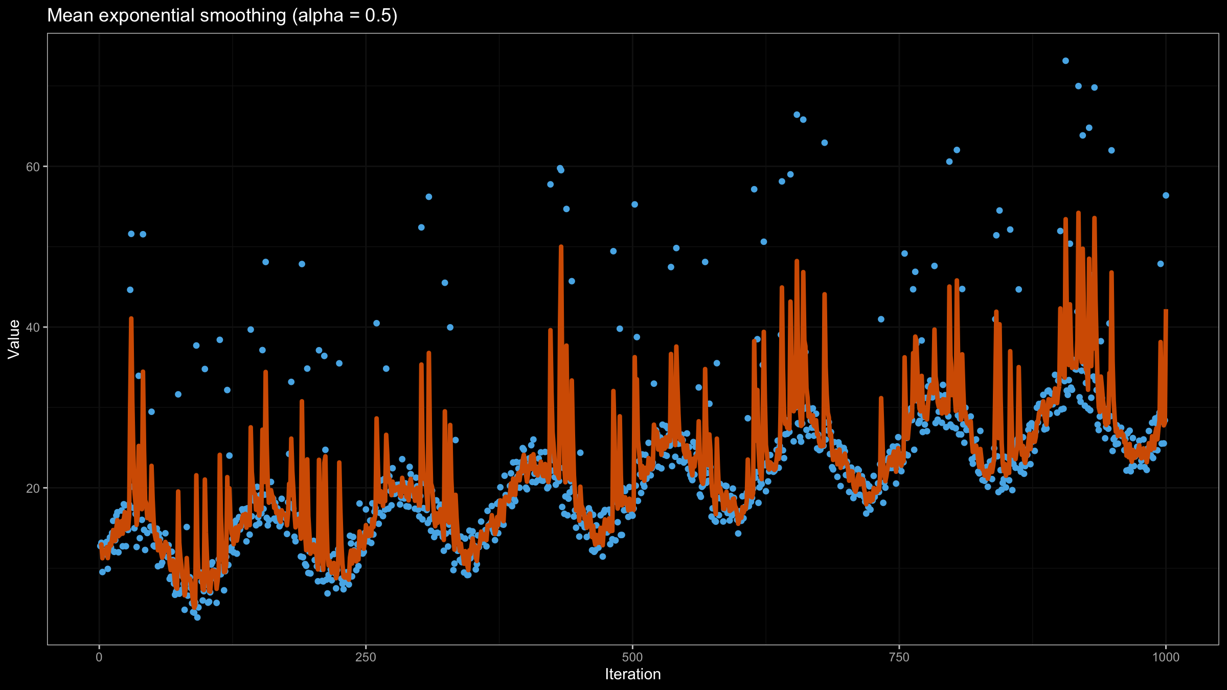
It looks a little bit better, but we still have too many “poor” values. Let’s try to reduce the value of $\alpha$ to $0.1$:
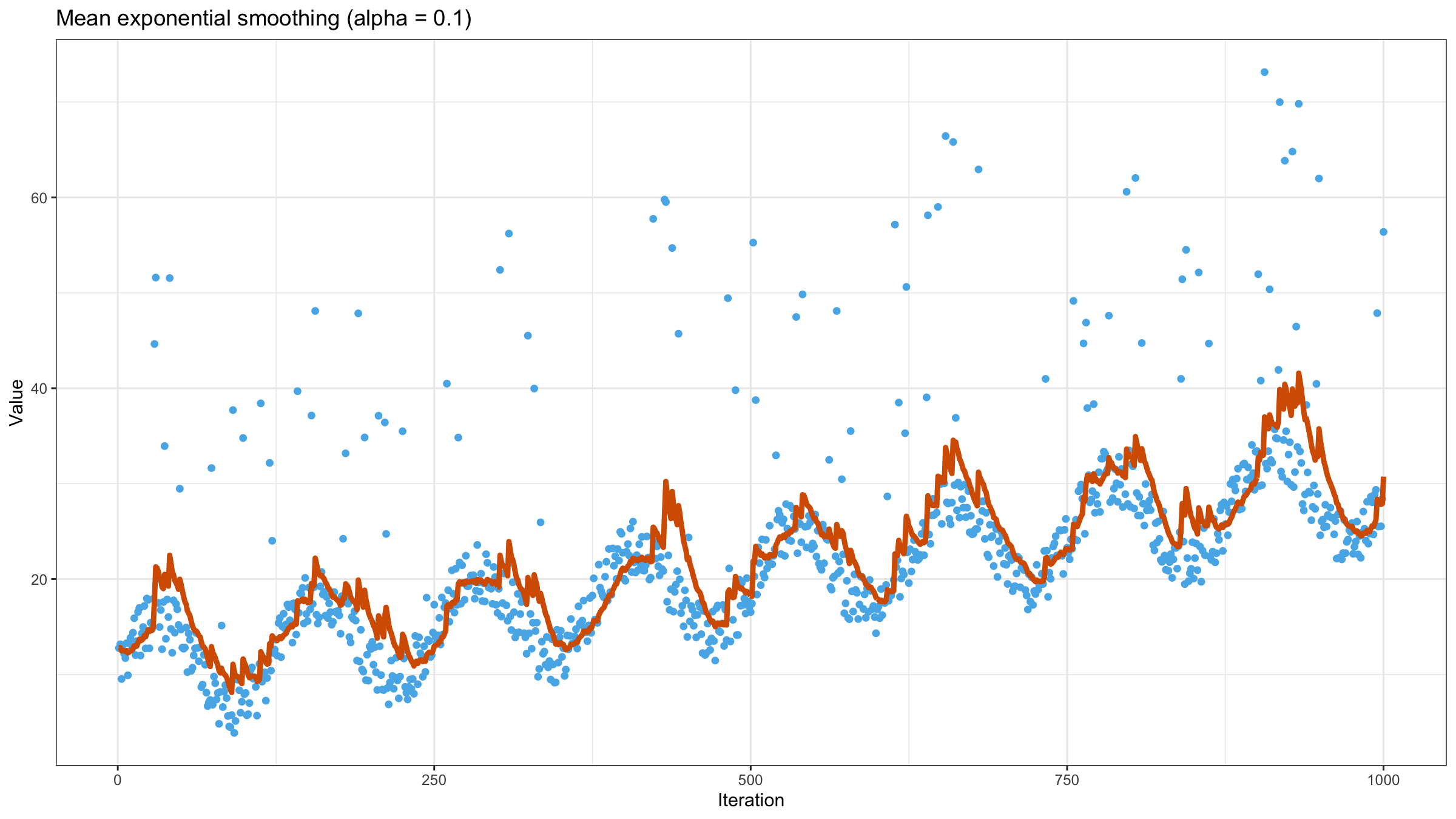
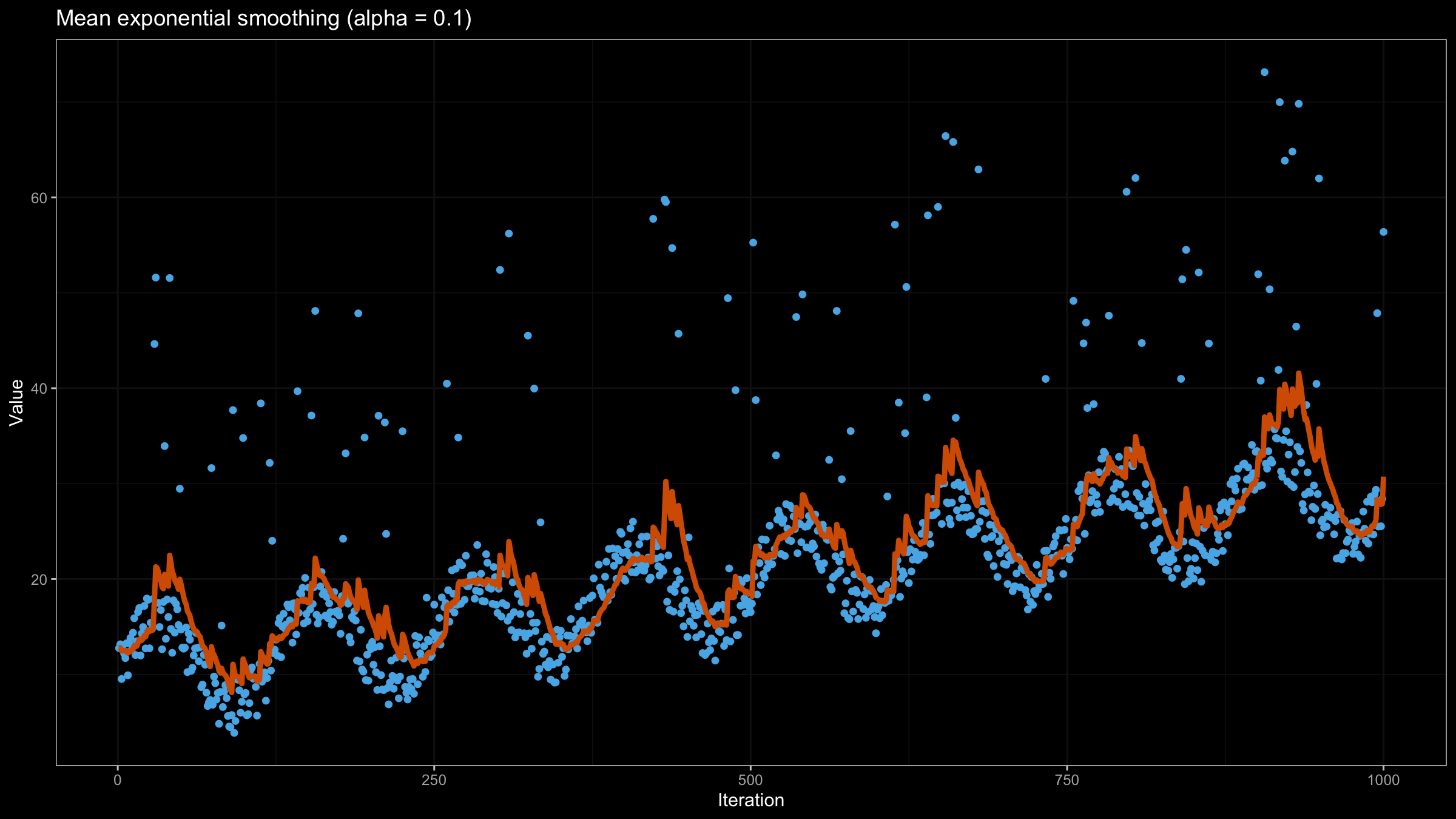
Now it looks much better, but the line is still not so smooth. It’s not a problem of exponential smoothing, it’s a problem of the mean as a measure of central tendency. When the underlying distribution has a heavy tail (and the corresponding samples have extreme outliers), the mean is not a good way to estimate the “average.” Let’s consider the density plot of the Pareto distribution ($x_m = 1, \alpha = 1.05$):
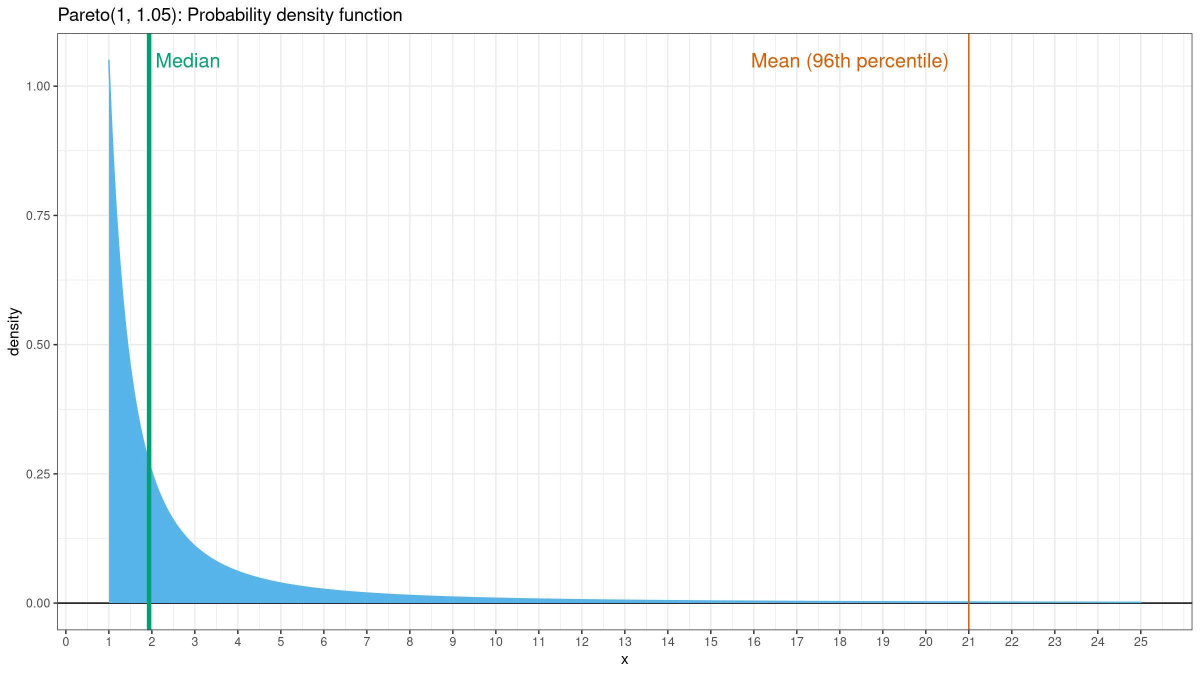
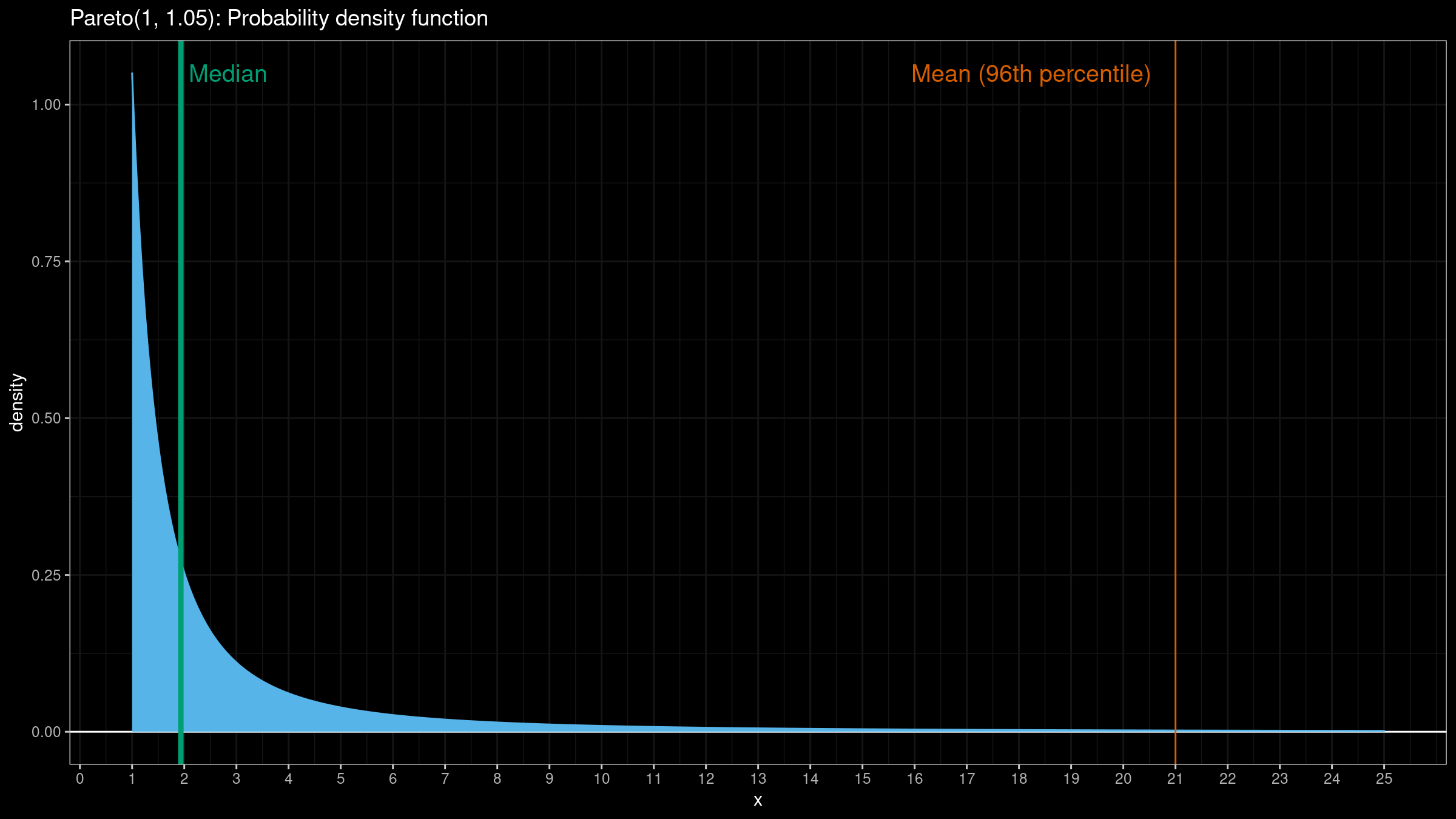
For this distribution, the mean value is about the $96^\textrm{th}$ percentile. This value is pretty far from the most significant part of the distribution. In such cases, the median is a more stable and more acceptable choice of the “average” metric.
Quantile exponential smoothing
To estimate distribution quantiles, we will use the Harrell-Davis quantile estimator because it’s much more efficient than the traditional quantile estimators. If we want to get a better robustness level, we can also consider the winsorized and trimmed modifications of the Harrell-Davis quantile estimator (the corresponding efficiency overview can be found here).
The easiest way to assign exponential weights to our observations is exponential decay. If we want to assign weights $w$ for observations $\{ x_1, \ldots, x_n \}$, we can use the following equation:
$$ w_t = e^{-\lambda (n-t)} $$where $\lambda$ is the decay constant. In order to set the $\lambda$ value, we can express it via the half-life value $t_{1/2}$:
$$ \lambda = \frac{\ln(2)}{t_{1/2}}. $$The half-life gives us a nice property of the weight function: $w_{i-t_{1/2}} = 0.5 w_i$. Thus,
$$ w_n = 1, \quad w_{n-t_{1/2}} = 0.5, \quad w_{n-2t_{1/2}} = 0.25, \quad w_{n-3t_{1/2}} = 0.125, \quad \ldots $$Once we defined the weight function, the Harrell-Davis quantile estimation $q^*_p$ of the $p^\textrm{th}$ quantile can be expressed as follows (the complete overview of this method can be found here):
$$ q^*_p = \sum_{i=1}^{n} W^*_{i} \cdot x_i,\quad W^*_{i} = I_{r^*_i}(a^*, b^*) - I_{l^*_i}(a^*, b^*), $$$$ \left\{ \begin{array}{rcc} l^*_i & = & \dfrac{s_{i-1}(w)}{s_n(w)},\\ r^*_i & = & \dfrac{s_i(w)}{s_n(w)}, \end{array} \right. $$$$ s_i(w) = \sum_{j=1}^i w_j, $$$$ \left\{ \begin{array}{rccl} a^* = & p & \cdot & (n^* + 1),\\ b^* = & (1-p) & \cdot & (n^* + 1), \end{array} \right. $$$$ n^* = \frac{\Big( \sum_{i=1}^n w_i \Big)^2}{\sum_{i=1}^n w_i^2 } $$where $I_t(a, b)$ is the regularized incomplete beta function.
The corresponding confidence interval can also be estimated using the modification of the Maritz-Jarrett method for weighted samples.
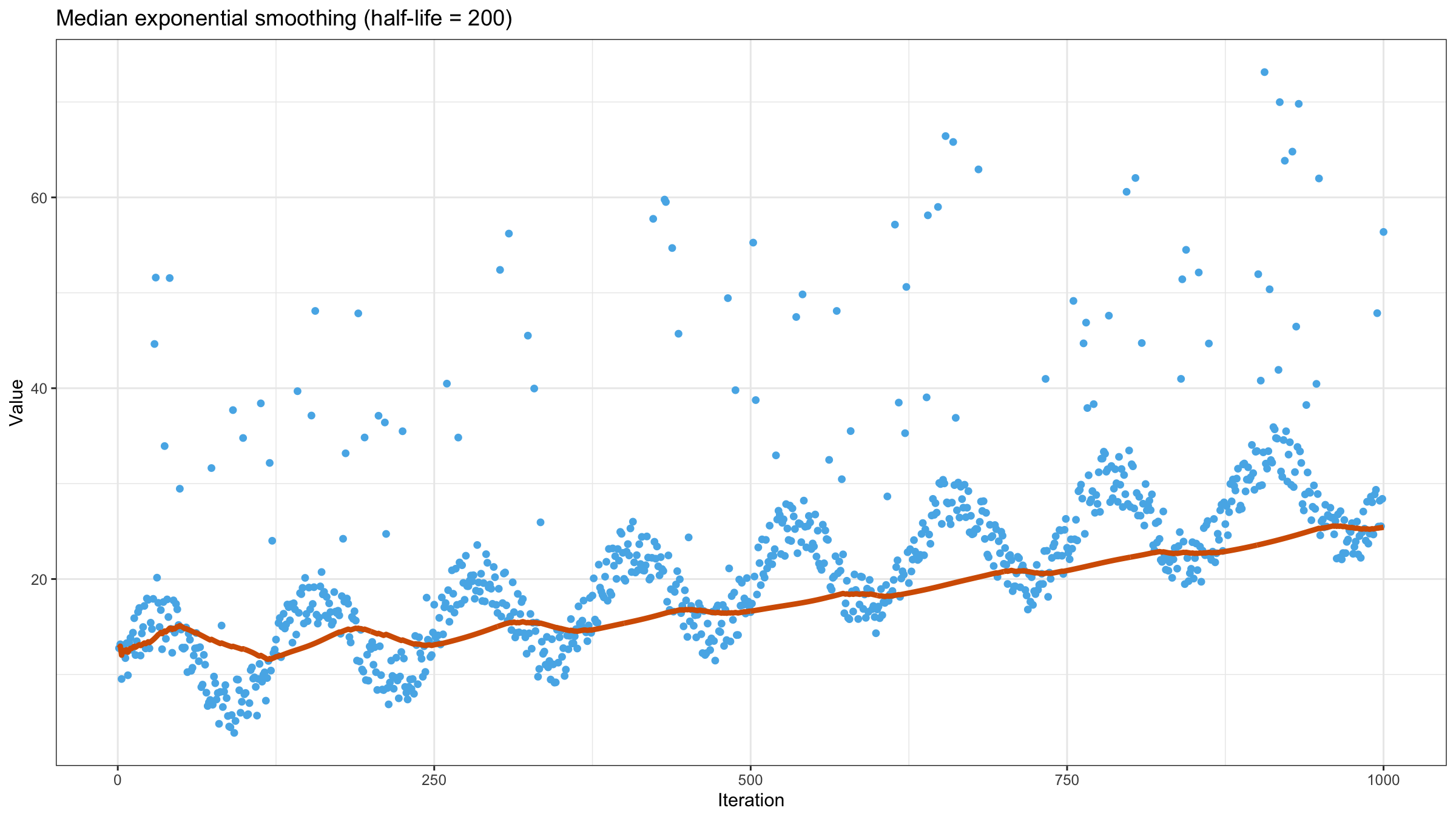
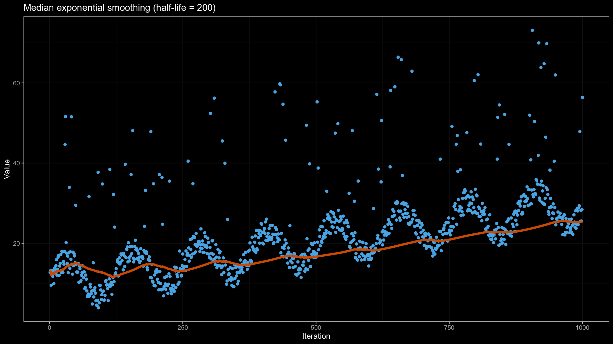
Now let’s try to apply the above equation to our data set using $\textrm{half-life} = 10$:
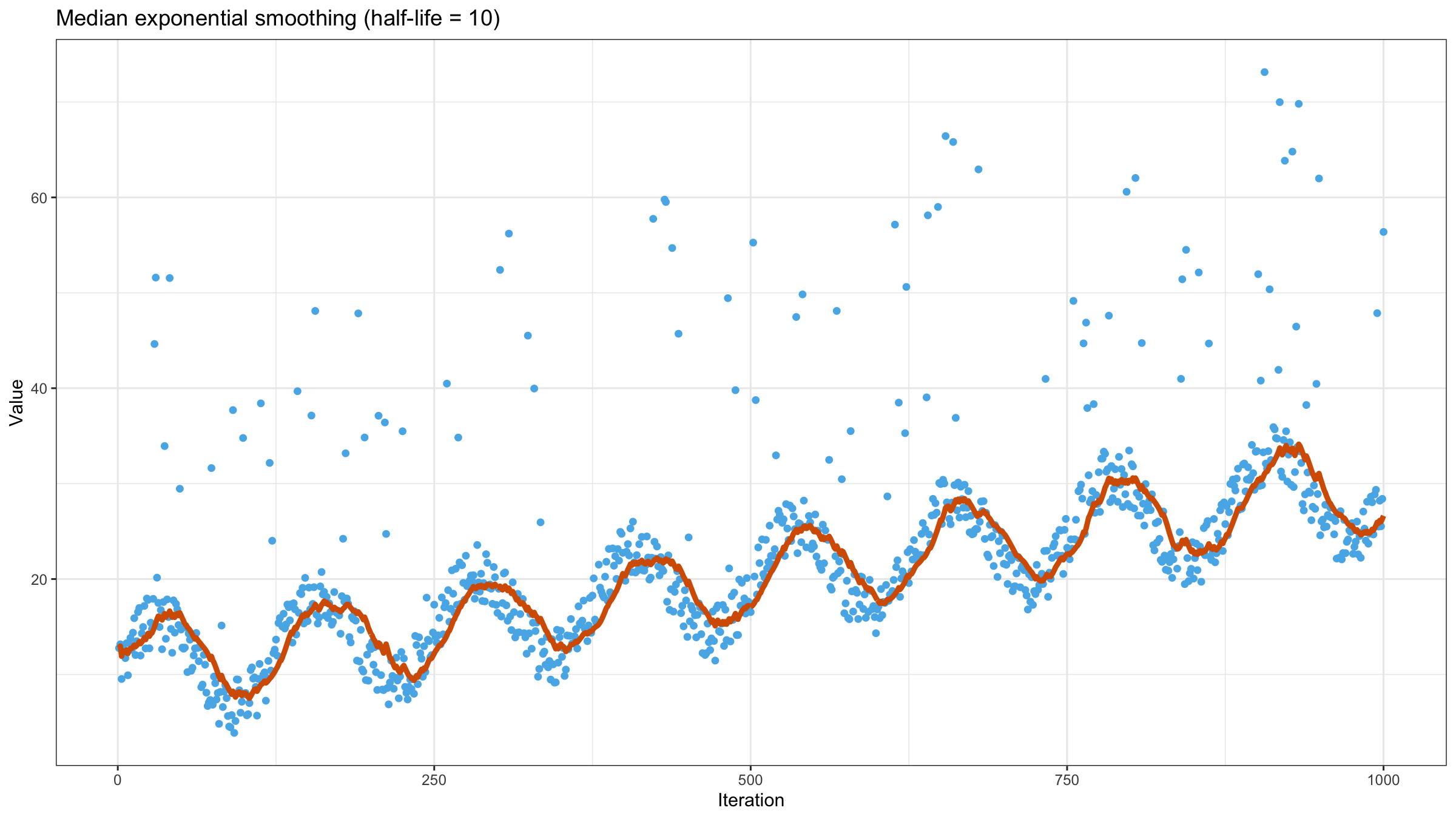
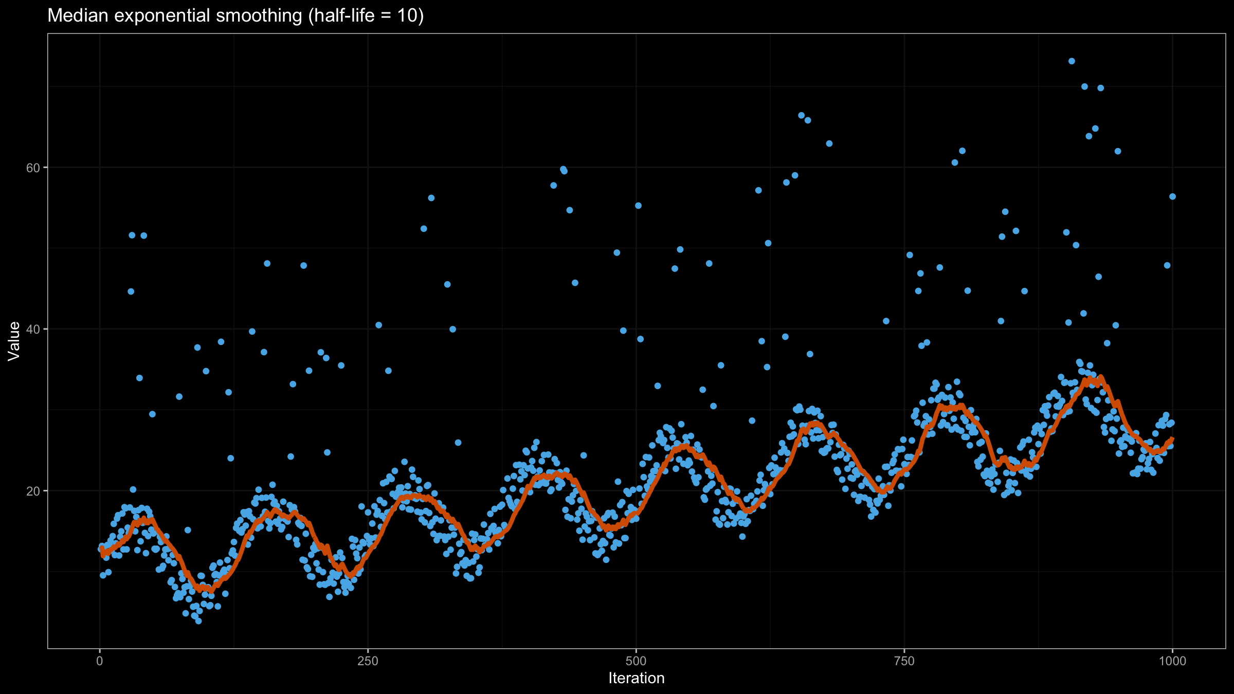
Increasing the half-life value gives more smooth but less adaptive line:
Incremental implementation of quantile exponential smoothing
The most significant advantage of the exponentially weighted moving mean is its computational efficiency: it can be recalculated using $O(1)$ complexity based on the previous value. In the case of quantile exponential smoothing, we can’t do it using $O(1)$ complexity because we need a sorted array of values to estimate the quantile value. To improve the algorithm performance, we can use a data structure that allows maintaining a sorted version of $\{ x_i \}$ with $O(\log n)$ update operation (e.g., a balanced binary tree). However, the Harrell-Davis quantile estimator still has $O(n)$ complexity. This also can be improved using the winsorized and trimmed modifications of the Harrell-Davis quantile estimator
Conclusion
In this post, we discussed quantile exponential smoothing using the exponentially weighted moving Harrell-Davis quantile estimations. This approach allows getting the moving quantile values that are more stable and smooth than the classic exponentially weighted mean values. The only disadvantage of this method is its computational complexity which is $O(n)$ for each estimated value.