Rethinking Type I/II error rates with power curves

When it comes to the analysis of a statistical significance test design, many people tend to overfocus purely on the Type I error rate. Those who are aware of the importance of power analysis often stop at expressing the Type II error rate as a single number. It is better than nothing, but such an approach always confuses me.

Let us say that the declared Type II error rate is 20% (or the declared statistical power is 80%). What does it actually mean? If the sample size and the significance level (or any other significance criteria) are given, the Type II error rate is a function of the effect size. When we express the Type II error rate as a single number, we always (implicitly or explicitly) assume the target effect size. In most cases, it is an arbitrary number that is somehow chosen to reflect our expectations of the “reasonable” effect size. However, the actual Type II error rate and the corresponding statistical power depend on the actual effect size that we do not know. Some researchers estimate the Type II error rate / statistical power using the measured effect size, but it does not make a lot of sense since it does not provide new information in addition to the measured effect size or p-value. In reality, we have high statistical power (low Type II error rate) for large effect sizes and low statistical power (high Type II error rate) for small effect sizes. Without the knowledge of the actual effect size (which we do not have), the Type II error rate expressed as a single number mostly describes this arbitrarily chosen expected effect size, rather than the actual properties of our statistical test.

A similar problem arises with the Type I error rate. I believe that working with the traditional nil hypothesis (that assumes that the effect size is exactly zero) or other kinds of point hypotheses (that compare the effect size with an exact number) are meaningless. In real life, nil hypotheses are almost always wrong. Any kind of changes in the experimental setup almost always have an impact on the measurements. And it is almost impossible to design such an experiment in which two tested distributions are identical with an infinite level of precision. Therefore, it is always possible to detect a statistically significant difference if we can indefinitely increase the sample size. A reasonable solution to this problem is switching to the null hypothesis that assumes that the effect size is negligible. This approach has multiple names: practical significance tests, minimum-effect tests, equivalence tests, and so on. Regardless of the name, the null hypothesis now covers a range of effect sizes that are marked as non-significant. When we operate with the word “negligible”, we tend to think that this range is so small that we can act like it is almost a point. However, such an assumption is often misleading. In order to solve the described nil hypothesis problem, this “negligible” range should be reasonably large. Thus, the classic definition of the Type I error rate (positive rate for the case when the effect size is zero) stops being fully applicable. Indeed, the positive rate for the zero effect size case describes only a single point of the “negligible” range. Since we extended the null hypothesis assumption, we also extended the bounds of Type I errors. If the true effect size falls within the “negligible” range, but it is not exactly zero, the actual positive rate will be different from the classic Type I error rate for zero effect size.

Thus, when we express Type I and Type II error rates as two numbers, such an approach can be misleading since it does not provide the full picture. Also, this makes it much more difficult to compare different statistical tests in terms of statistical significance and power, if these tests use different “negligible” ranges for Type I errors or different “expected” effect sizes for Type II errors.

Power curve by effect size

So, what can we do to resolve the described problem with the classic Type I/II error rates? I would like to share an approach that I use to compare various test procedures. Instead of focusing on separate numbers for specific effect sizes, I evaluate the whole function that describes the dependency of the positive detection rate on the actual effect size. Sometimes, such a function is referenced as the power curve by effect size (e.g., see bartlett2022).

Let me demonstrate this approach using a classic example. We compare two samples from two normal distributions $\mathcal{N}(\mu_1, 1)$ and $\mathcal{N}(\mu_2, 1)$ and we want to check if there is a difference between their means $\mu_1$ and $\mu_2$. We try to use the classic one-tailed Student’s t-test and the one-tailed Mann–Whitney U test with the classic nil hypothesis that states that there is no difference between distributions. In our experiment, we set the statistical significance level to the notorious $\alpha = 0.05$.

In order to evaluate the properties of each test, we do the following:

• Enumerate various actual effect sizes $d$;
• For each effect size $d$, we generate pairs of random samples from $\mathcal{N}(0, 1)$ and $\mathcal{N}(d, 1)$; for each pair, we perform both statistical tests and check if they return a positive result respecting the given $\alpha = 0.05$;
• Repeat the previous step multiple times so that we can evaluate the probability of getting the positive result for the given effect size $d$ using the Monte-Carlo method;
• Build a power curve plot that demonstrates the dependency of the positive detection rate on the actual effect size.

Below, you can see the results for the sample size $n=10$:

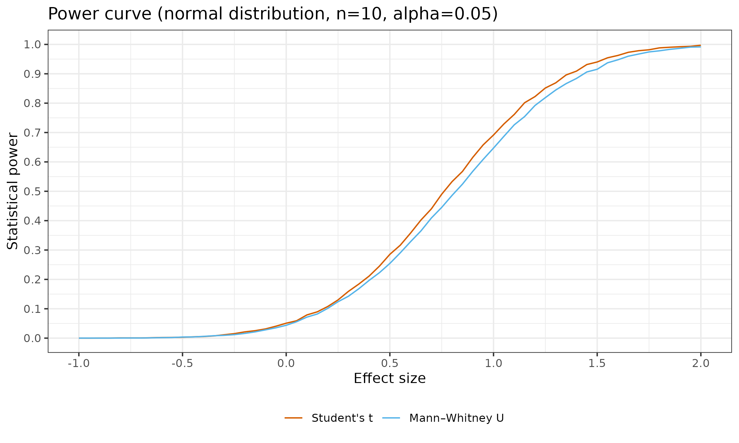
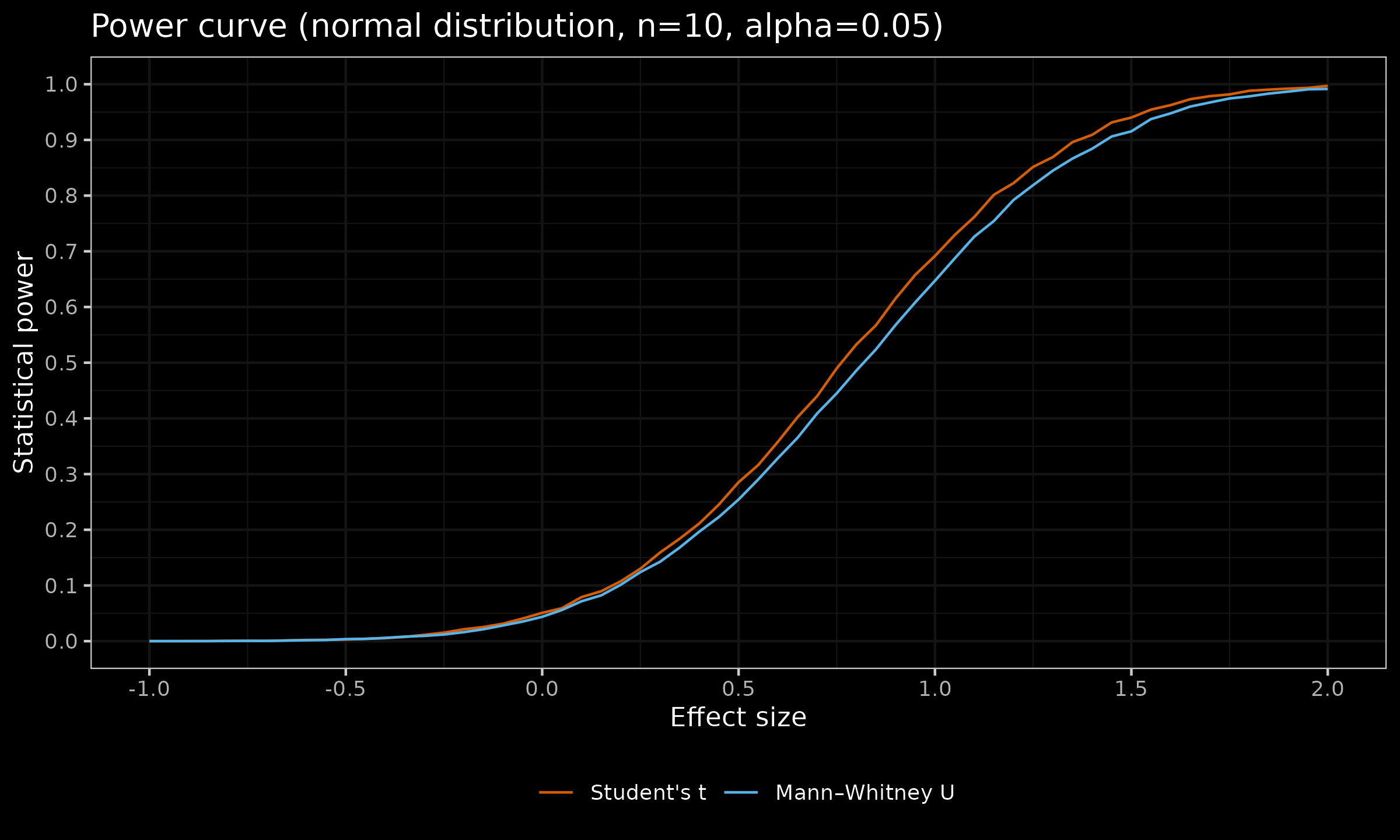
Here are some relevant observations:

• For the zero effect size, the positive rate is 0.05, which matches the specified $\alpha = 0.05$ (the “classic” Type I error rate).
• For the positive effect sizes, these charts show the corresponding statistical power of the two tests. As we can see, in the context of the considered problem, the Student’s t-test is more powerful than the Mann–Whitney U test. This matches our expectations since the Student’s t-test assumes normality (and this assumption is valid) and therefore has more information about the given samples (unlike the Mann–Whitney U test that does not have the normality assumption).
• While the Mann–Whitney U test is less powerful, the actual difference between the powers of these two tests is not so big. To be more specific, in the given experiment, the maximum observed difference of $\approx 0.05$ appears for $d = 0.95$. For large and small effect sizes, the observed difference is even smaller: for $d<0$ or $d>2$ it is less than $\approx 0.007$.
• The transition from the Student’s t-test to the Mann–Whitney U test is a reasonable switch if we expect a deviation from normality expressed in the form of occasional outliers. However, such a switch reduces the statistical power of the testing procedure. Using the above chart, we can see the exact power loss for the whole range of various effect sizes.

Now let us look at the similar plots for $n \in \{ 20, 30, 100 \}$:

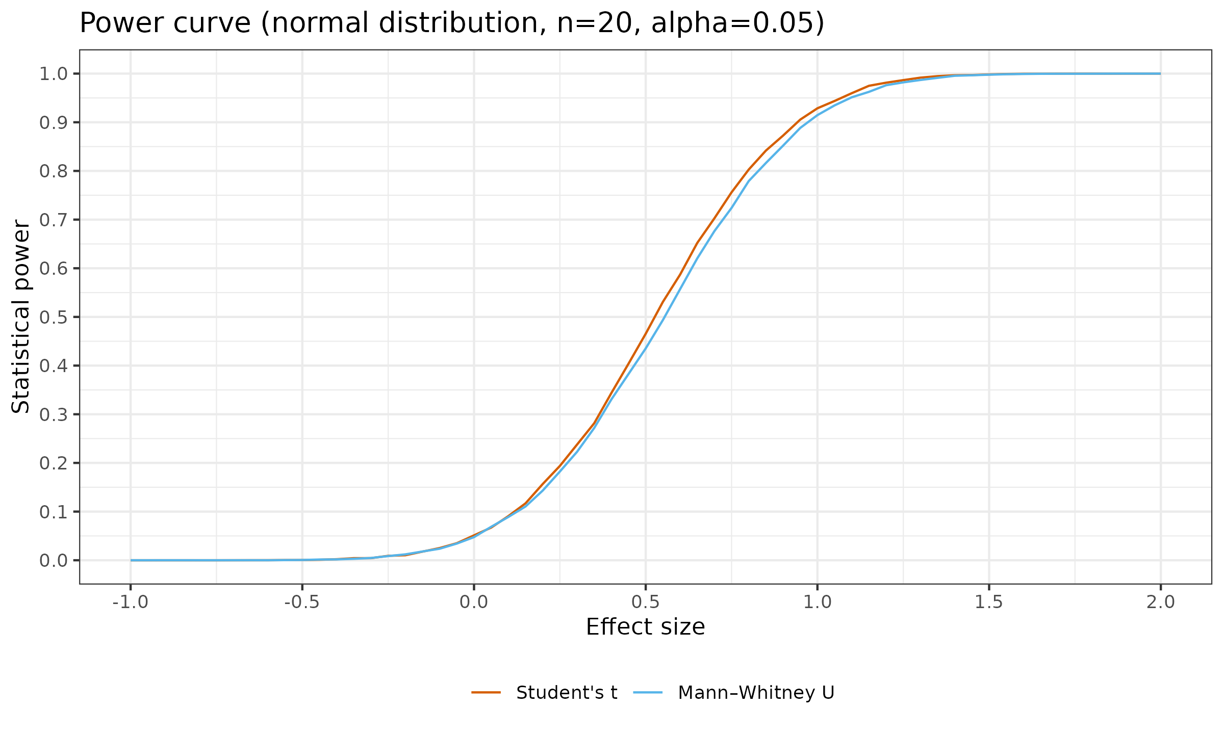
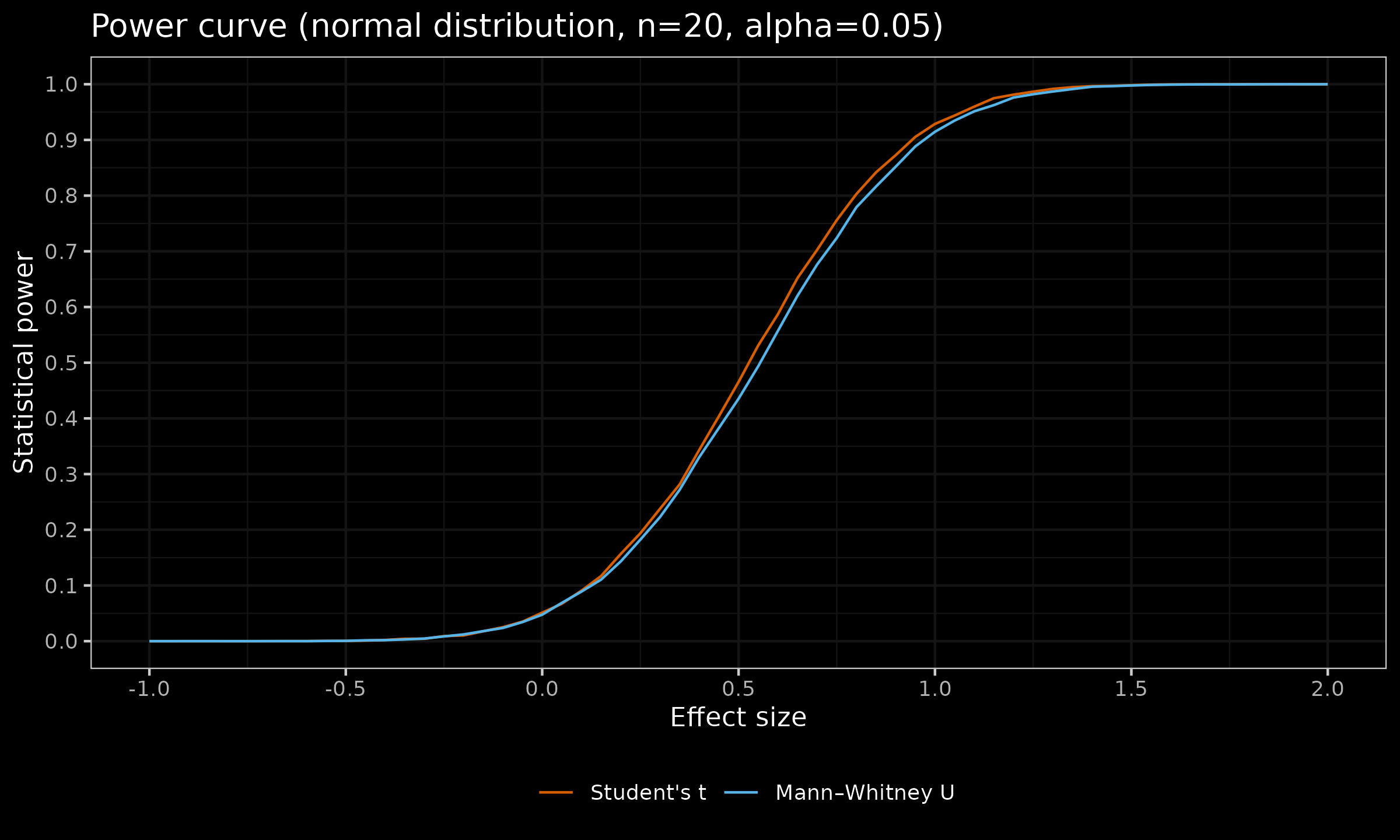
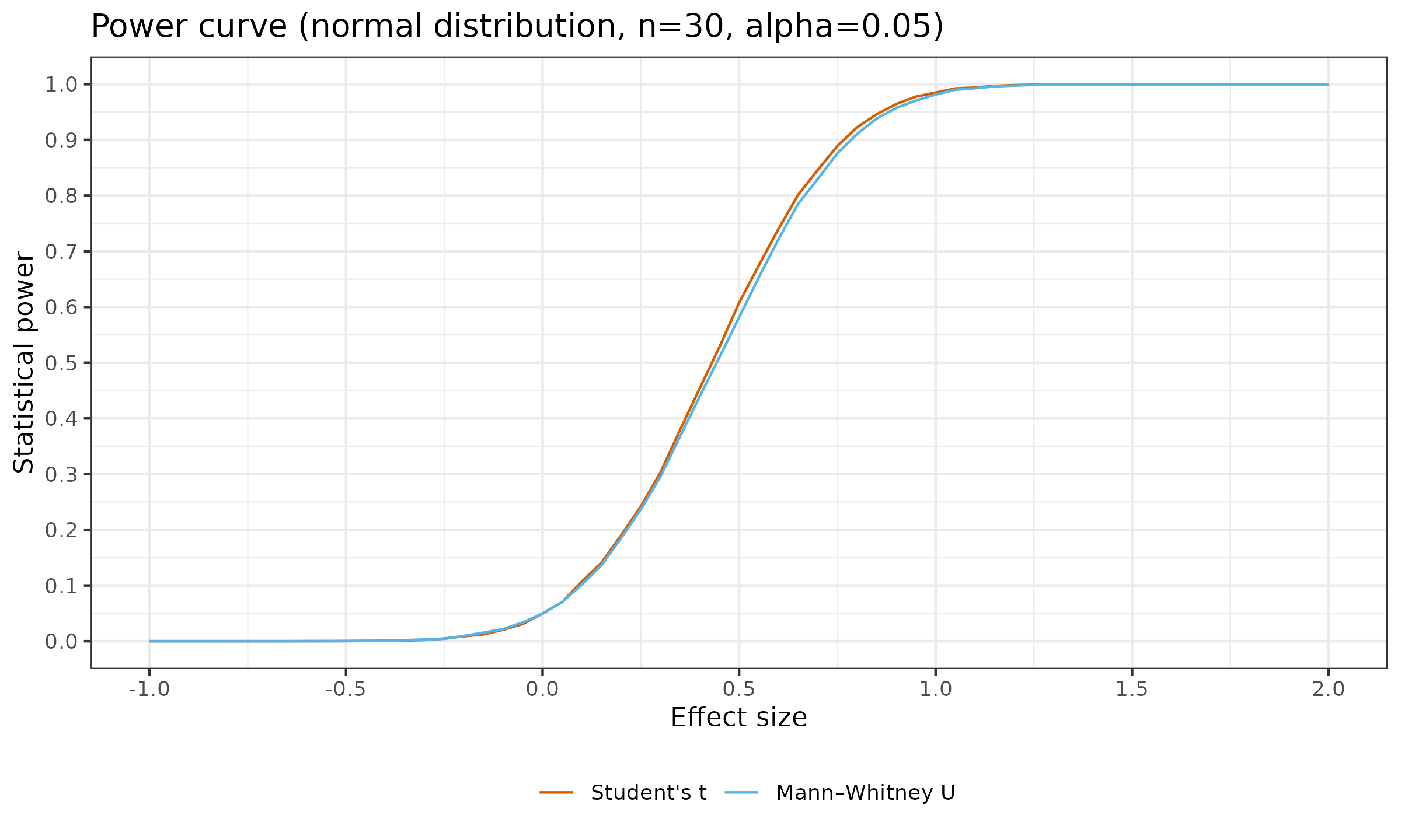
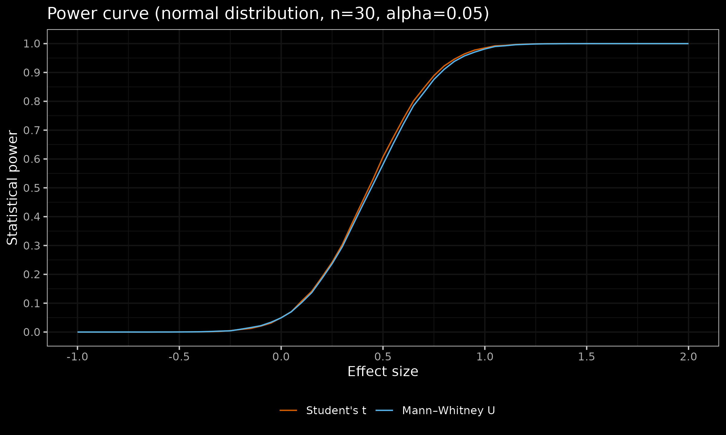
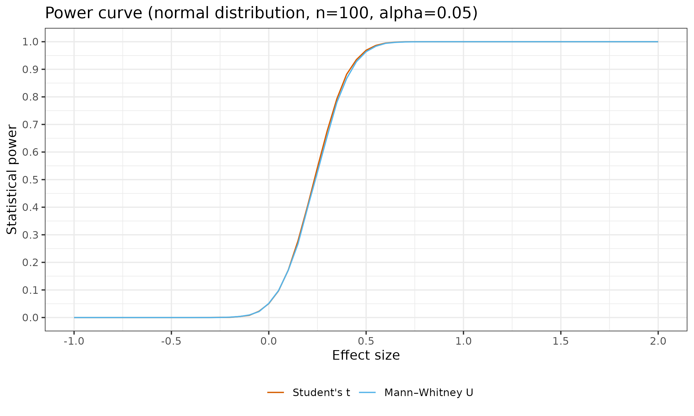
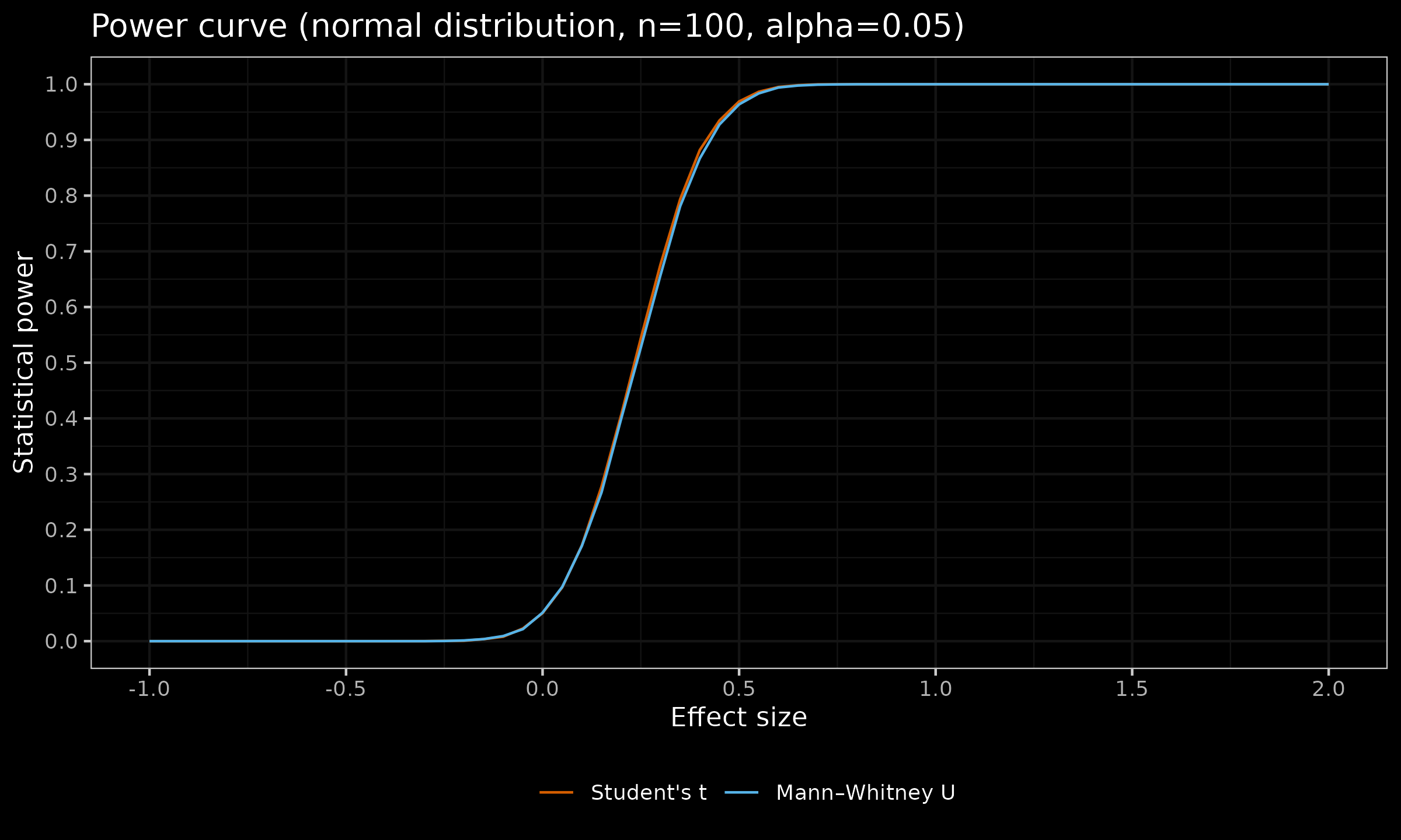
As we can see, with larger sample sizes, the difference in the statistical power between the considered tests almost disappears. For $n=100$, the maximum observed difference of $\approx 0.02$ appears for $d = 0.3$ (for $d<0$ or $d>0.65$, the difference is less than $\approx 0.0008$).

Conclusion

While the suggested approach of analyzing the power curves is more complicated than the classic Type I/II error rate (it forces you to consider the whole function instead of two numbers), I believe that it reduces the level of misleadingness and helps to improve the testing procedure design.