Resistance to the low-density regions: the Harrell-Davis median
In the previous post, we defined the resistance function that show sensitivity of the given estimator to the low-density regions. We also showed the resistance function plots for the mean and the sample median. In this post, we explore corresponding plots for the Harrell-Davis median.
The resistance function
As was shown in the previous post, we define the function of resistance to the low-density regions as follows:
$$ R(T, n, s) = \max_{s \leq k \leq n} R(T, n, s, k), $$$$ R(T, n, s, k) = |T(\mathbf{x}_k) - T(\mathbf{x}_{k-s})|, $$$$ \mathbf{x}_k = \{ \underbrace{0, 0, \ldots, 0}_{k}, \underbrace{1, 1, \ldots, 1}_{n-k} \}, $$where $T$ is an estimator, $n$ is the sample size, $s$ is the number of sample values that jump from the first mode to the second one.
Resistance of the Harrell-Davis median
Now it’s time to build the plot of $R(T, n, s)$ that compares the mean, the sample median, and the Harrell-Davis median. In this experiment, we consider $n \leq 100$, $s \in \{1, 2, 3, 4, 5, 6\}$. Here are the plots:
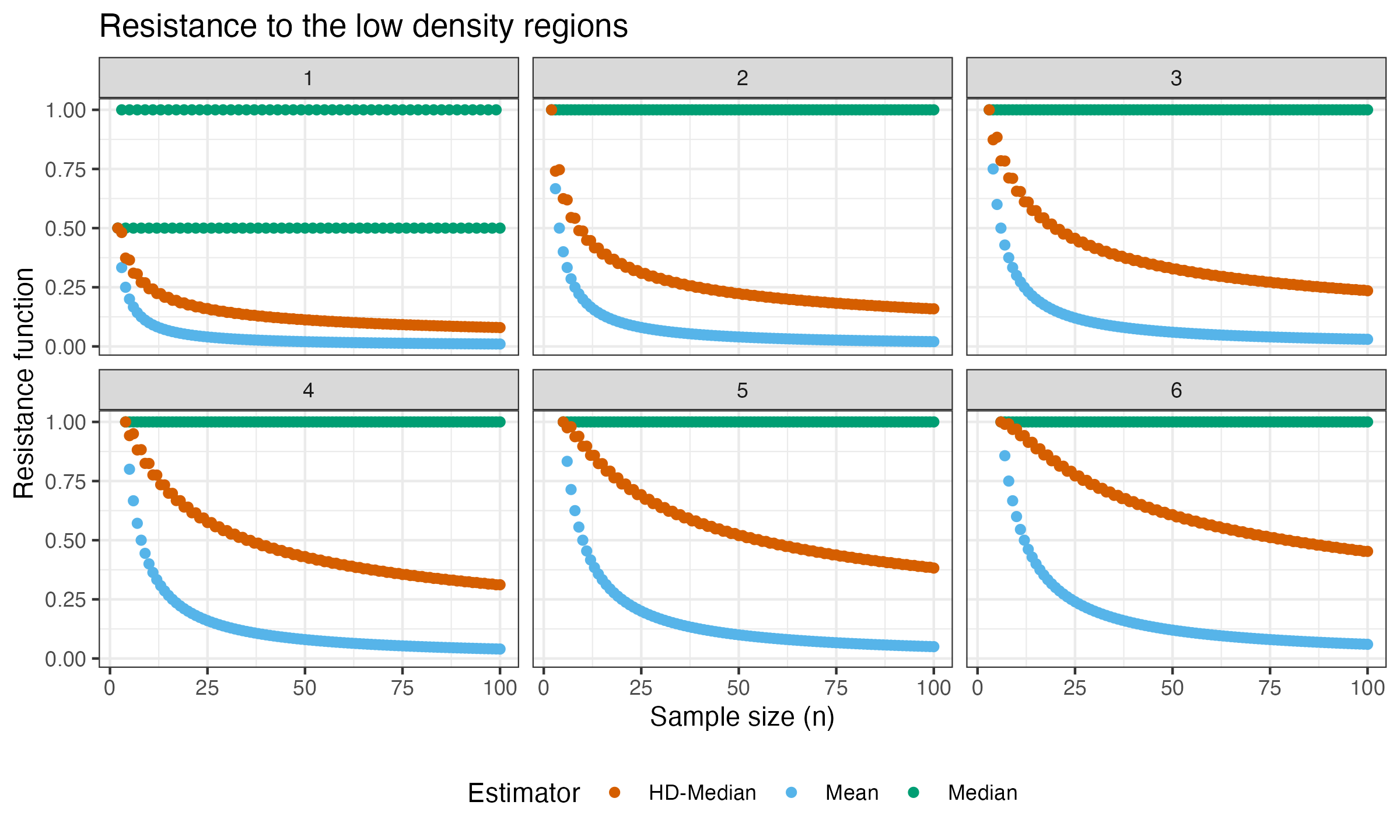

As we can see, the Harrell-Davis median is not only more statistically efficient to low-density regions, but it is also more resistant to the low-density regions.
In future posts, we will explore the resistance function for other measures of central tendency.