Resistance to the low-density regions: the mean and the median
When we discuss resistant statistics, we typically assume resistance to extreme values. However, extreme values are not the only problem source that can violate usual assumptions about expected metric distribution. The low-density regions which often arise in multimodal distributions can also corrupt the results of the statistical analysis. In this post, I discuss this problem and introduce a measure of resistance to low-density regions.
Median sampling distribution
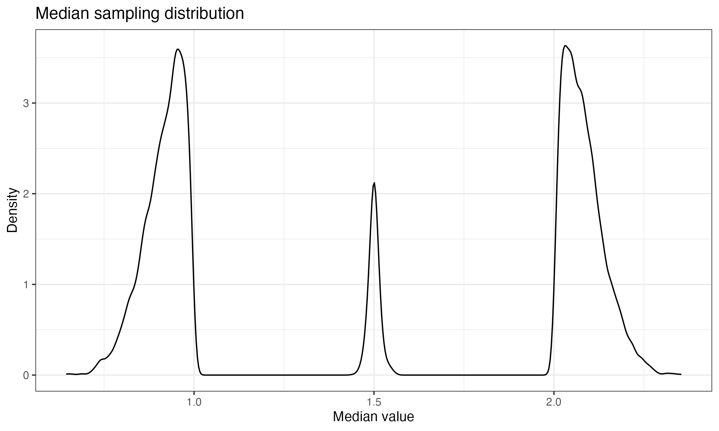
In most cases, the median sampling distribution is asymptotically normal with mean $M$ and variance $1/(4nf^2(M))$, where $n$ is the number of elements in samples, $f$ is the probability density function of the original distribution, and $M$ is the true median of the original distribution. As I have already discussed, this rule doesn’t always work. To be specific, the asymptotic variance $1/(4nf^2(M))$ is not defined when $f(M) = 0$. For example, let us consider the median sampling distribution for a mixture of two unimodal distributions $\mathcal{U}(0, 1)$ and $\mathcal{U}(2, 3)$:


And here is the corresponding median sampling distribution (10000 samples of size 100):

The resistance function
In order to define a function that describes resistance to the low-density regions, we consider an ultimate case that illustrates the problem: the Bernoulli distribution. It is a discrete distribution that gives $0$ with probability $p$ and $1$ with probability $1-p$. It can be considered as a condensed version of a bimodal distribution: $0$ is the first mode, $1$ is the second mode; the $(0;1)$ interval is the low density region (the density is zero within this interval).
If we are interested in a stable reproducible metric, we should expect small changes in the metric values when a single sample value or a few sample values “jump” from one mode to another. More formally, let $T$ be an estimator, $n$ be a sample size, $s$ be a number of sample values that jump from the first mode to the second one. Let’s build a function that shows the changes in the estimator value during such a jump. We denote a sample that contains $k$ zeros and $n-k$ ones as $\mathbf{x}_k$:
$$ \mathbf{x}_k = \{ \underbrace{0, 0, \ldots, 0}_{k}, \underbrace{1, 1, \ldots, 1}_{n-k} \} $$If $s \leq k$ sample values jump from the first mode to the second one, the estimation change is defined by the following function:
$$ R(T, n, s, k) = |T(\mathbf{x}_k) - T(\mathbf{x}_{k-s})|. $$If we don’t know the exact value of $k$, but we want to evaluate the maximum possible change, we can define another function:
$$ R(T, n, s) = \max_{s \leq k \leq n} R(T, n, s, k). $$Now let us explore this function for the mean and for the median.
Resistance of the mean and the median
Now let’s build the plot of $R(T, n, s)$ for the mean and the median. In this experiment, we consider $n \leq 100$, $s \in \{1, 2, 3, 4, 5, 6\}$. Here are the plots:
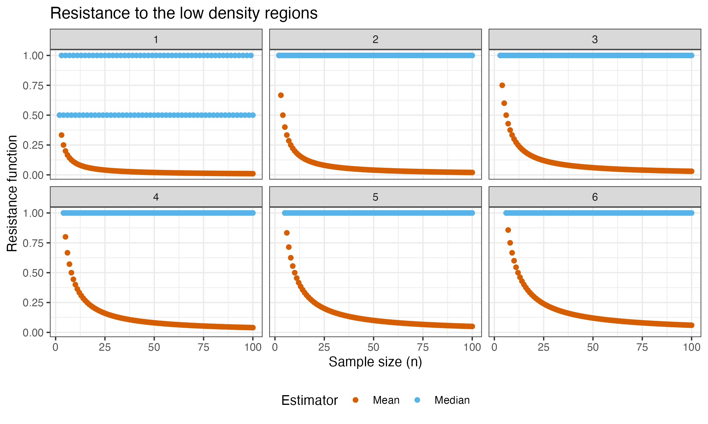
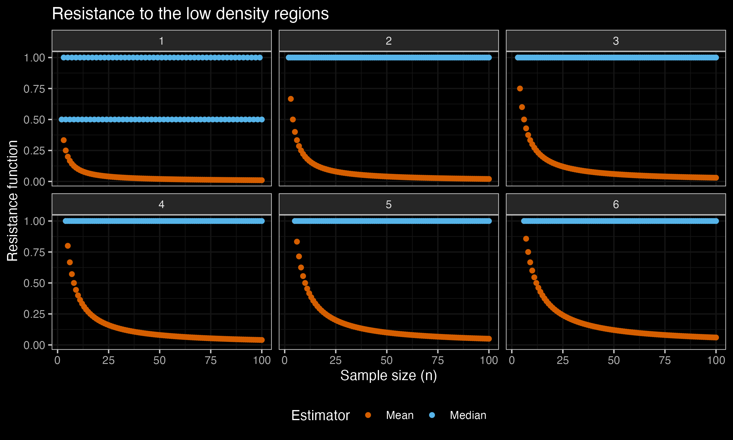
As we can see, the mean is quite resistant to the low-density regions, while it’s not robust (its breakdown point is zero). Meanwhile, the median is not resistant to the low-density regions (for $s\geq 2$, $R(\operatorname{median}, n, s) = 1$, which is the maximum value of $R(T, n, s)$), while it’s extremely robust (its breakdown point is 0.5).
In future posts, we will explore the resistance function for other measures of central tendency.