Median vs. Hodges-Lehmann: compare efficiency under heavy-tailedness
In the previous post, I shared some thoughts on how to evaluate the statistical efficiency of estimators under heavy-tailed distributions. In this post, I apply the described ideas to actually compare efficiency values of the Mean, the Sample Median, and the Hodges-Lehmann EstimatorHodges-Lehmann location estimator under various distributions.
Classic statistical efficiency
We start with the definition of the classic relative statistical efficiency. Let us say we have two estimators $T_1$ and $T_2$. For the given sample $\mathbf{x} = (x_1, x_2, \ldots, x_n)$, they provide estimations of a parameter. Let $\theta$ be the true value of the parameter. The relative efficiency of these estimators is defined as
$$ \operatorname{eff}(T_1, T_2) = \frac{\mathbb{E}[(T_2-\theta)^2]}{\mathbb{E}[(T_1-\theta)^2]}. $$If $T_1$ and $T_2$ are unbiased estimators, the above expression can be simplified as follows:
$$ \operatorname{eff}(T_1, T_2) = \frac{\mathbb{V}[T_2]}{\mathbb{V}[T_1]}. $$Robust statistical efficiency
The problem with the above definition is that it includes the variance $\mathbb{V}$ which is not robust. There are two popular efficient robust alternatives to the variance:
- Shamos EstimatorShamos Estimator: $\operatorname{Quantile}(|x_i-x_j|_{i < j}, 0.5) \cdot C_1$
- Rousseeuw–Croux $Q_n$ estimator: $\operatorname{Quantile}(|x_i-x_j|_{i < j}, 0.25) \cdot C_2$
These values are $50^\textrm{th}$ and $25^\textrm{th}$ percentiles of the $|x_i-x_j|_{i < j}$ distribution. Such percentile orders look quite arbitrary. Under the normal distribution, the choice of the exact percentile order is not so important: all of them are proportional to the true variance values. In the nonparametric case, the choice of the percentile order is determined by the desired values of the breakdown point and the Gaussian efficiency. However, we we consider severe deviations from normality, a single value of this distribution doesn’t provide the full picture. Therefore, it could mislead us and we can come up with wrong conclusions. What if we consider not a single quantile value, but the whole distribution? We can define such an efficiency function as follows:
$$ \operatorname{eff}(T_1, T_2, p) = \frac{\operatorname{Quantile}(\operatorname{APD}(T_2), p)}{\operatorname{Quantile}(\operatorname{APD}(T_1), p)}, $$where $\operatorname{APD}$ is the distribution of absolute pairwise differences between obtained estimations. Let us try to apply this approach!
Numerical simulations
We consider the following distributions:
- (Light-tailed) The standard uniform distribution $\mathcal{U}(0, 1)$
- (Light-tailed) The standard normal distribution $\mathcal{N}(0, 1)$
- (Light-tailed) The standard exponential distribution $\operatorname{Exp}(1)$
- (Heavy-tailed) The standard log-normal distribution
- (Heavy-tailed) The Weibull distribution with $\textrm{shape} = 0.5$
- (Heavy-tailed) The standard Cauchy distribution
For each distribution, we compare the relative efficiency of the Median and the Hodges-Lehmann location estimator ($\operatorname{HL}$) to the Mean. Here are the results:
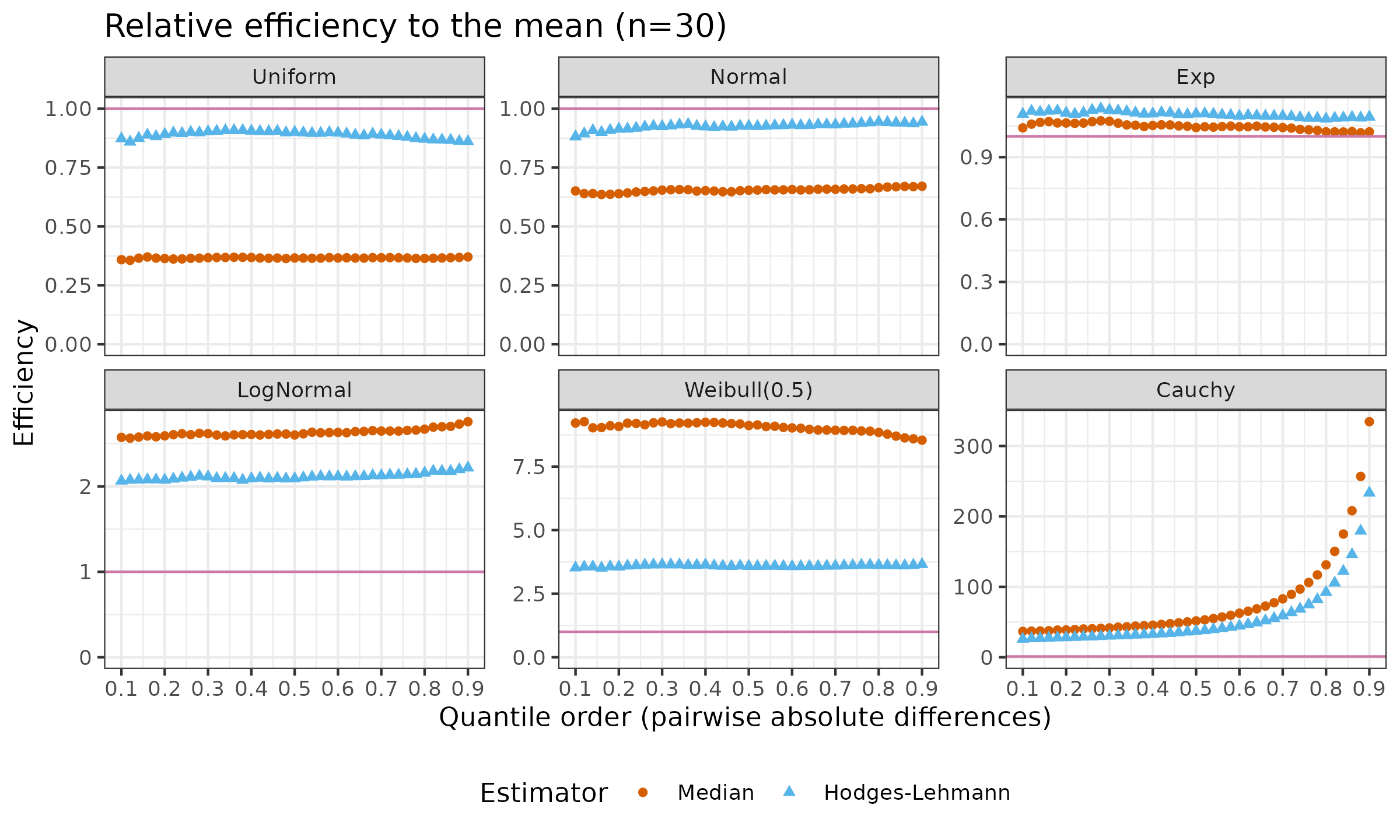
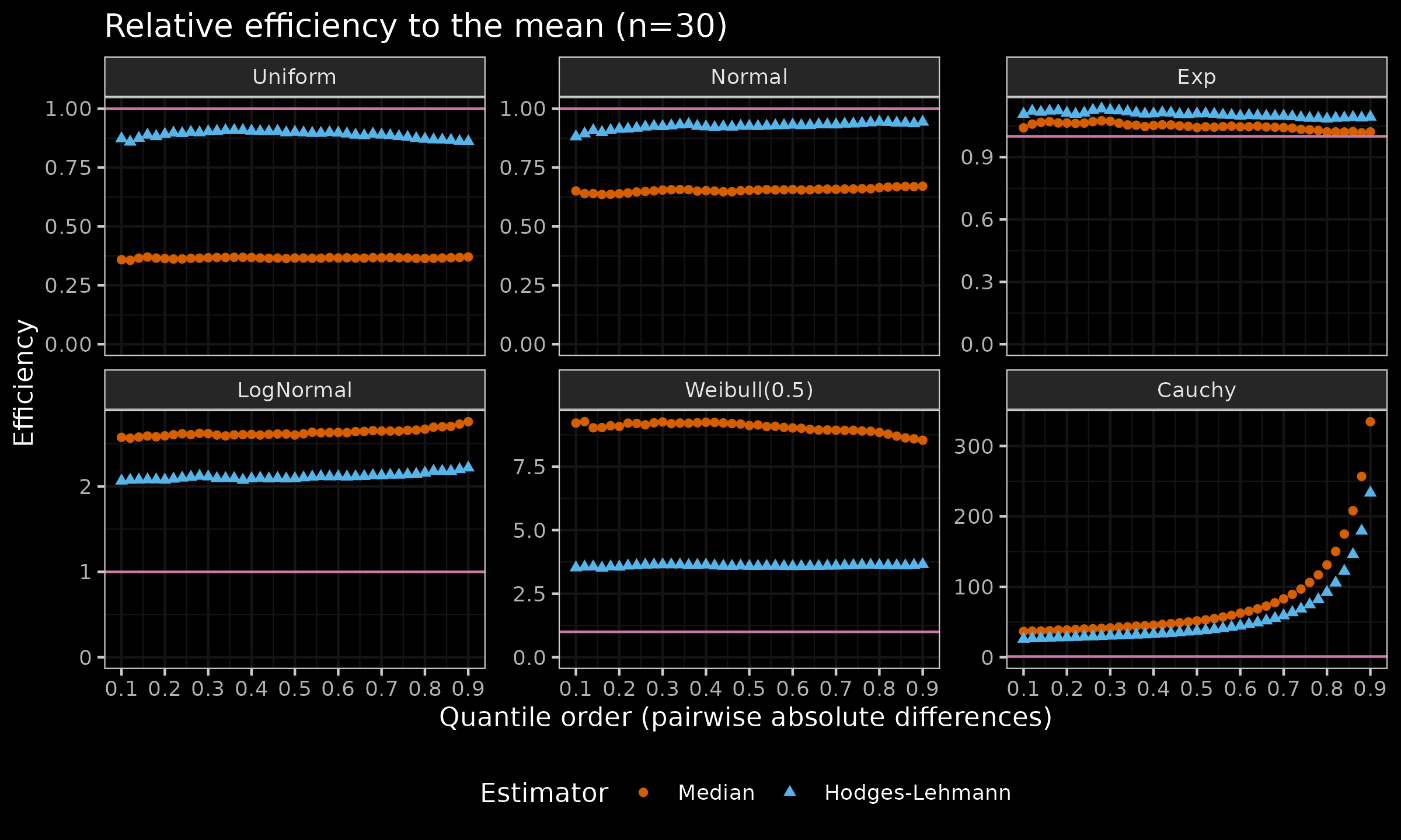
As we can see, for the light-tailed distributions, $\operatorname{HL}$ is more efficient than the Median. While we enlarge the distribution tail $\left(\mathcal{U}(0, 1) \to \mathcal{N}(0, 1) \to \operatorname{Exp}(1)\right)$, the difference in efficiency is decreasing. After the switch to the heavy-tailed distributions, the Median becomes the winner. This happens because the Median (the asymptotic breakdown point of $50\%$) is more robust than $\operatorname{HL}$ (the asymptotic breakdown point of $29\%$). The heavier the tail, the larger the observed difference.
The plot for the Cauchy distribution is especially interesting. While the efficiency function for the first five distributions looks almost like a constant, for the Cauchy distribution, we can see an obviously heavily increasing efficiency function. The choice of $p$ has a significant impact on the efficiency values: it starts at $30..40$ for small $p$ and ends at $200..300$ for large $p$.
Therefore, such an approach allows us to reveal the full efficiency picture and to get a more conscious choice of an appropriate estimator for our target distribution.