Robust alternative to statistical efficiency

Andrey Akinshin · 2021-06-01

Statistical efficiency is a common measure of the quality of an estimator. Typically, it’s expressed via the mean square error ($\operatorname{MSE}$). For the given estimator $T$ and the true parameter value $\theta$, the $\operatorname{MSE}$ can be expressed as follows:

$$ \operatorname{MSE}(T) = \operatorname{E}[(T-\theta)^2] $$

In numerical simulations, the $\operatorname{MSE}$ can’t be used as a robust metric because its breakdown point is zero (a corruption of a single measurement leads to a corrupted result). Typically, it’s not a problem for light-tailed distributions. Unfortunately, in the heavy-tailed case, the $\operatorname{MSE}$ becomes an unreliable and unreproducible metric because it can be easily spoiled by a single outlier.

I suggest an alternative way to compare statistical estimators. Instead of using non-robust $\operatorname{MSE}$, we can use robust quantile estimations of the absolute error distribution. In this post, I want to share numerical simulations that show a problem of irreproducible $\operatorname{MSE}$ values and how they can be replaced by reproducible quantile values.

We are going to compare four quantile estimators:

hf7: the traditional quantile estimator (also known as the Hyndman-Fan Type 7, see hyndman1996)
hd: the Harrell-Davis quantile estimator (see harrell1982)
sv1: the first Sfakianakis-Verginis quantile estimator (see sfakianakis2008)
no: the Navruz-Özdemir quantile estimator (see navruz2020)

With these estimators, we are going to estimate the median of the following distributions:

The standard uniform distribution $\mathcal{U}(0, 1)$ (light-tailed)
The standard normal distribution $\mathcal{N}(0, 1)$ (light-tailed)
The pareto distribution $\textrm{Pareto}(x_m = 1, \alpha = 1)$ (heavy-tailed)

In each experiment, we generate 20'000 random samples, each sample contains exactly 3 elements. For each sample, we estimate the median using the current estimator. Next, we build the distribution of absolute errors between the obtained median estimations and the true median value. For each absolute error distribution, we estimate all the quantile values and draw corresponding plots.

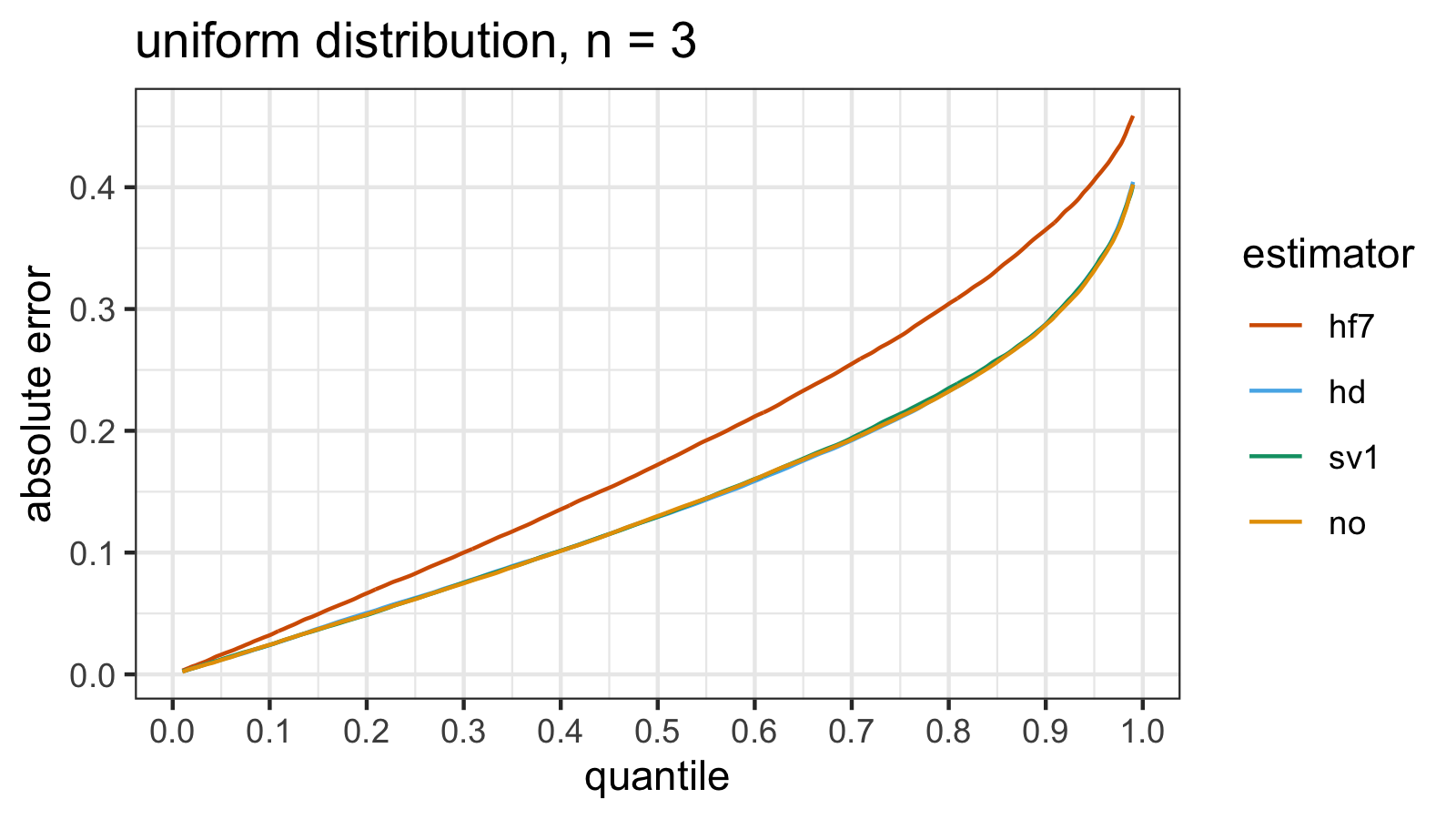
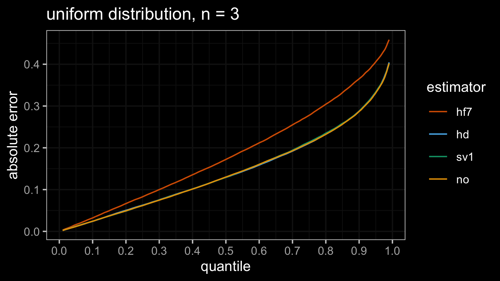
Uniform distribution

 estimator      mse      p25     p50     p75     p90     p95     p99
       hf7 0.049761 0.082785 0.17217 0.27775 0.36512 0.40580 0.45873
        hd 0.030902 0.062728 0.12931 0.21104 0.28773 0.33363 0.40441
       sv1 0.031096 0.062015 0.12936 0.21394 0.28739 0.33340 0.40215
        no 0.030811 0.061727 0.13005 0.21173 0.28704 0.33156 0.40228

In the case of standard uniform distribution, both the $\operatorname{MSE}$ and the absolute error quantile values provide consistent results. According to the simulations, hd/sv1/no perform much better than hf7. Meanwhile, we don’t see a noticeable difference between hd, sv1, and no.

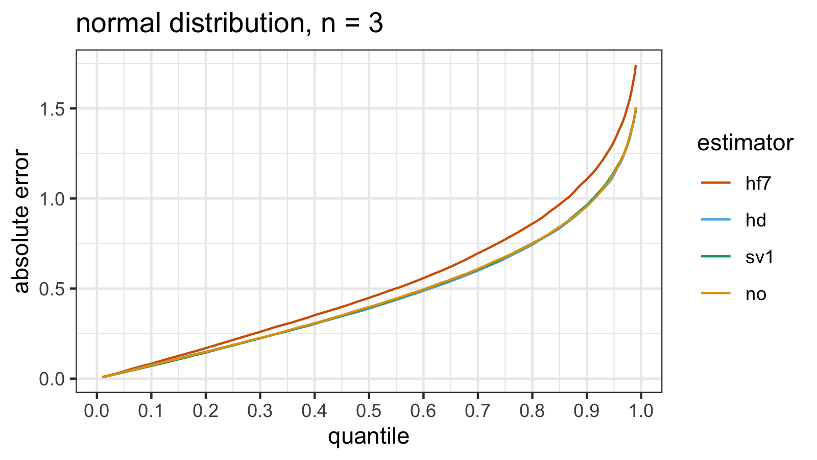
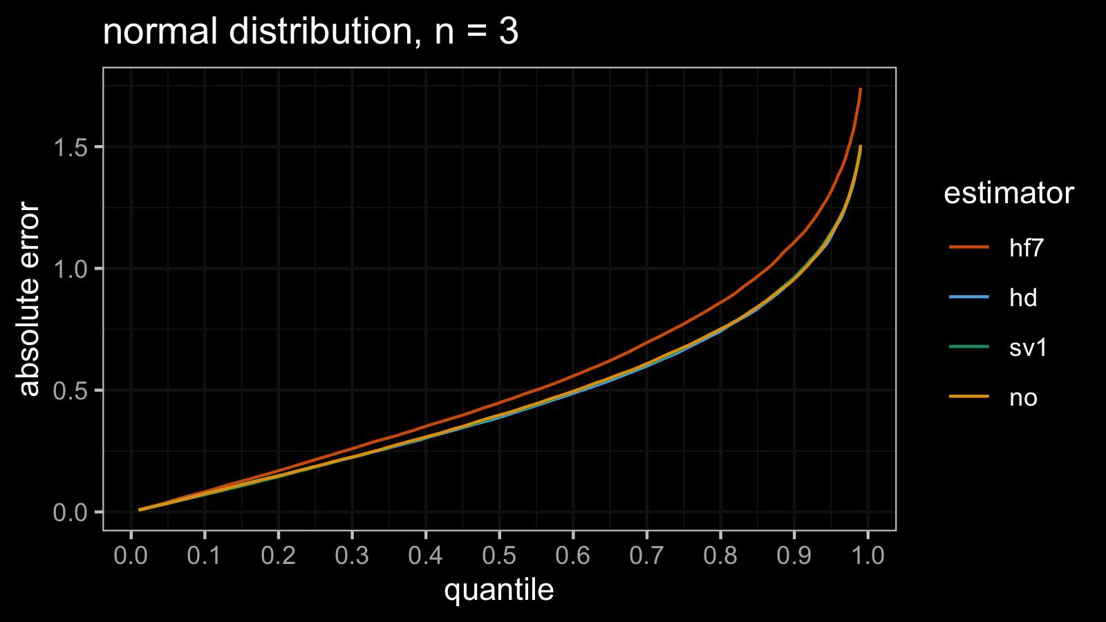
Normal distribution

 estimator     mse     p25     p50     p75     p90    p95    p99
       hf7 0.45162 0.21470 0.44859 0.77262 1.10815 1.3174 1.7413
        hd 0.33698 0.18662 0.38851 0.66673 0.96248 1.1328 1.4903
       sv1 0.34164 0.18439 0.39484 0.67337 0.96364 1.1482 1.4905
        no 0.34263 0.18713 0.39773 0.67639 0.95694 1.1420 1.5073

In the case of the standard normal distribution, we have a similar picture: the absolute error quantile values give the same overview of the quantile estimator efficiency as the $\operatorname{MSE}$.

Pareto distribution, attempt #1

It’s time to check a heavy-tailed distribution!

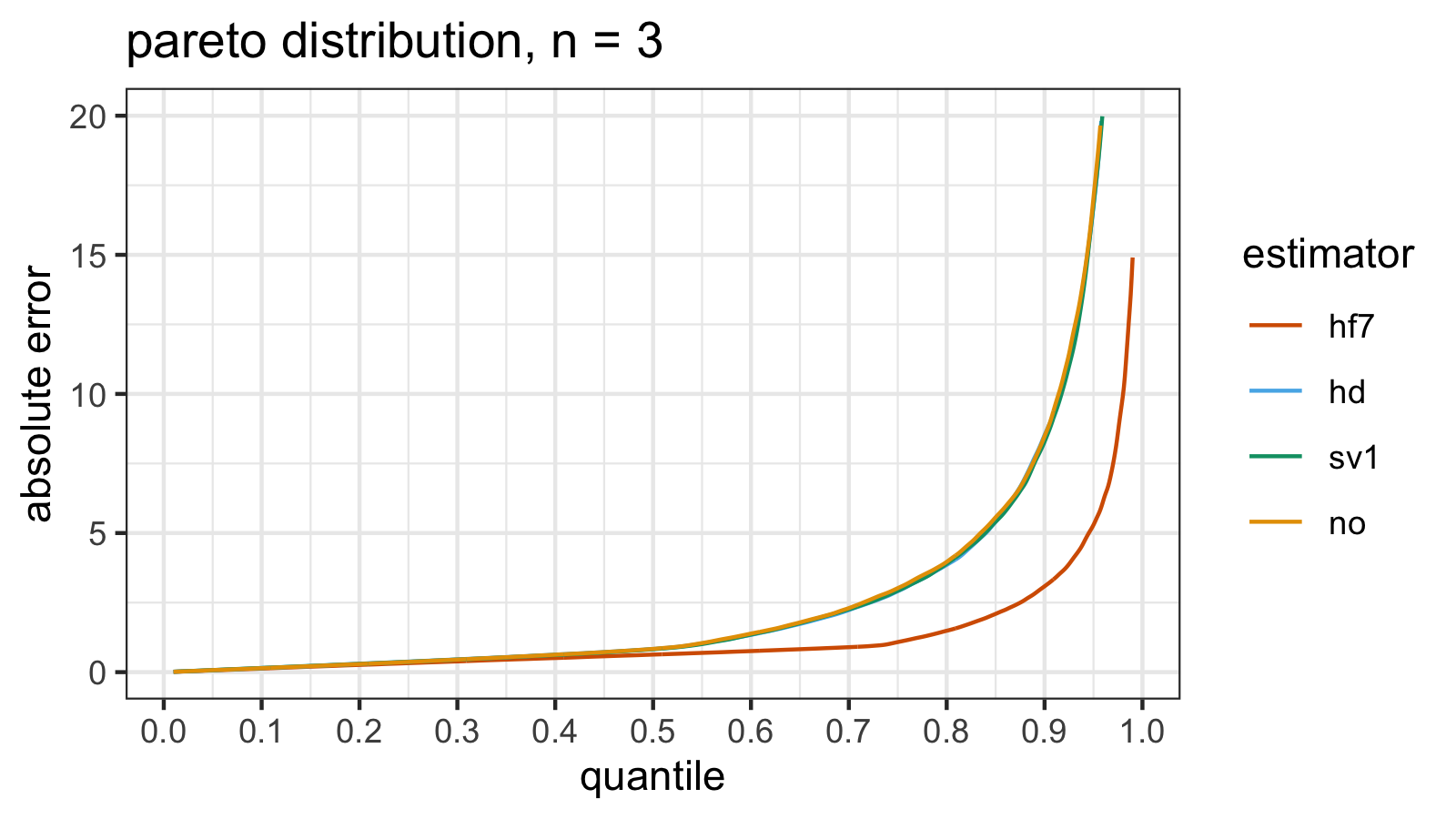
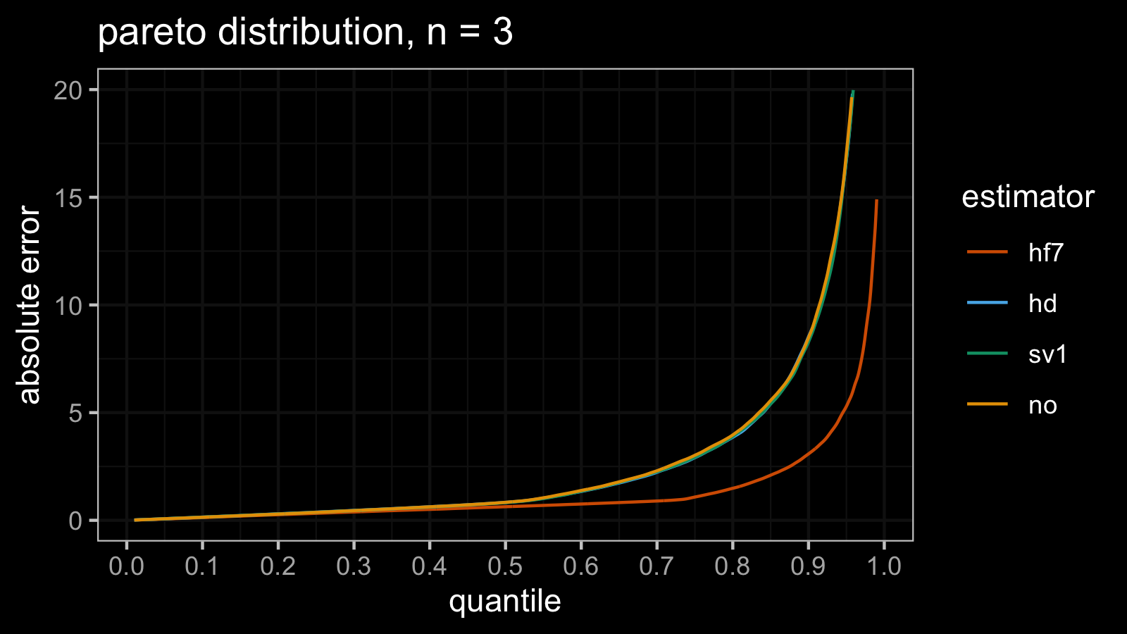
 estimator        mse     p25     p50    p75    p90    p95    p99
       hf7     31.978 0.32446 0.63152 1.0811 3.0858  5.293 14.905
        hd   2640.998 0.37870 0.83140 2.9100 8.5205 16.756 77.500
       sv1   9322.438 0.37274 0.82331 2.9271 8.2836 16.796 75.108
        no 128130.912 0.36925 0.83511 3.0203 8.4807 17.054 84.659

From the plot, we can see that hd/sv1/no perform the same way (worse than hf7): there is no noticeable difference between them. However, if we build an overview based on the $\operatorname{MSE}$ values, we get another conclusion. Let’s estimate the relative efficiency of hd, sv1, and no using hf7 as the baseline estimator:

$$ e(T_{\operatorname{HD}}) \approx \frac{31.978}{2640.998} \approx 0.0121 $$$$ e(T_{\operatorname{SV1}}) \approx \frac{31.978}{9322.438} \approx 0.0034 $$$$ e(T_{\operatorname{NO}}) \approx \frac{31.978}{128130.912} \approx 0.00025 $$

According to the $\operatorname{MSE}$ values, hd is 3.5 times better than sv1 and 48.5 times better than no!

Pareto distribution, attempt #2

Now let’s repeat the previous experiment with another set of random samples.

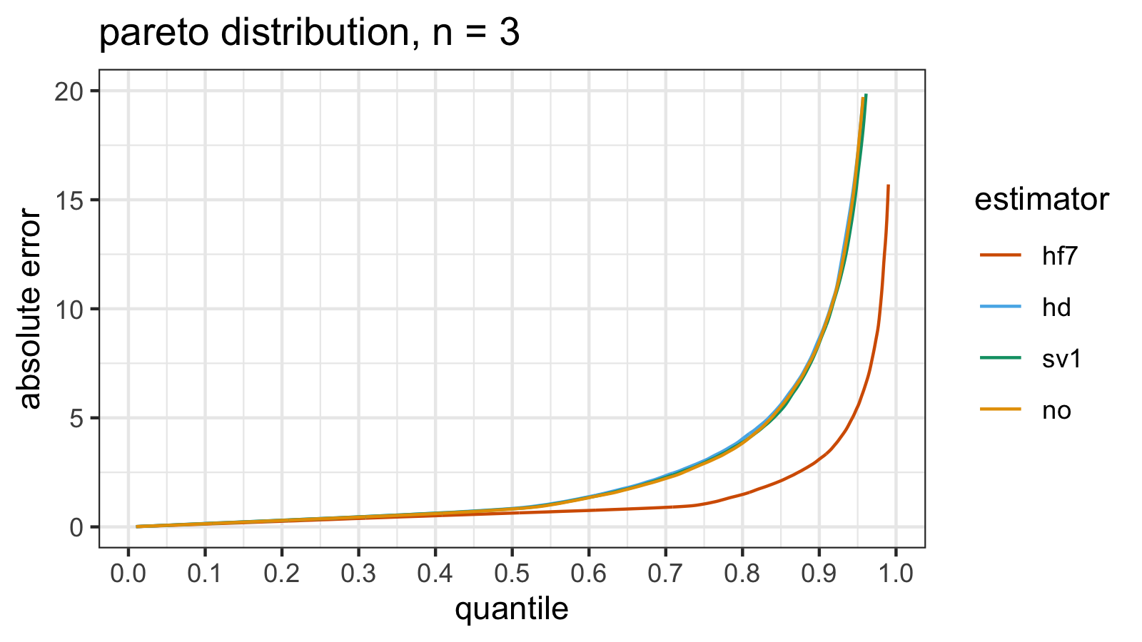
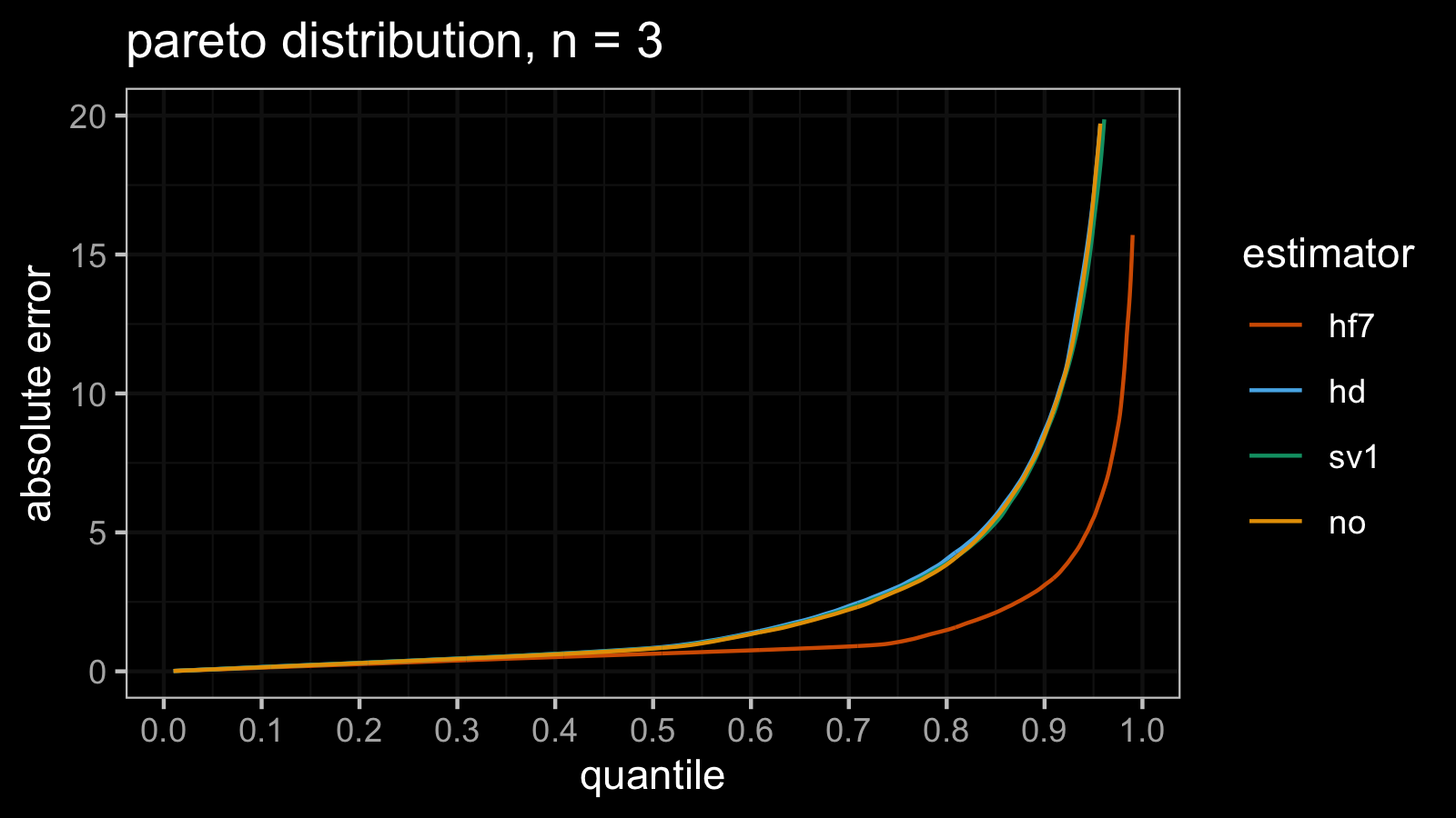
 estimator        mse     p25     p50    p75    p90     p95    p99
       hf7     27.384 0.32309 0.63282 1.0515 3.1039  5.5155 15.703
        hd 811526.384 0.38036 0.84433 3.0360 8.6536 17.0931 85.511
       sv1 718886.400 0.38023 0.82743 2.9420 8.4412 16.0745 71.577
        no  14857.025 0.37242 0.81987 2.9058 8.4988 17.0583 77.767

If we look at the absolute error quantile values, the second attempt is pretty similar to the first attempt. Of course, the numbers are not identical, but the difference is negligible. Such repeatability is impressive in the case of heavy-tailed distributions.

However, if we look at the $\operatorname{MSE}$ values, we can see that they are not so repeatable. Here are the relative efficiency values of hd, sv1, and no against hf7 in the second simulation:

$$ e(T_{\operatorname{HD}}) \approx \frac{27.384}{811526.38} \approx 0.000034 $$$$ e(T_{\operatorname{SV1}}) \approx \frac{27.384}{718886.400} \approx 0.000038 $$$$ e(T_{\operatorname{NO}}) \approx \frac{27.384}{14857.025} \approx 0.0018432 $$

Now the winner is no: it’s 54 times better than hd and 48 times better than sv1.

Pareto distribution, attempt #3

Let’s do the same experiment one more time.

 estimator       mse     p25     p50    p75    p90    p95    p99
       hf7     30.42 0.32526 0.63699 1.0355 3.0922  5.328 14.707
        hd 571078.71 0.37972 0.82261 2.9377 8.4516 16.400 75.704
       sv1 129449.18 0.37659 0.82254 2.8794 8.2823 16.356 84.715
        no   4729.29 0.38240 0.83073 2.9837 8.3501 16.606 74.399

Here are the updated $\operatorname{MSE}$-based relative efficiency values of hd, sv1, and no against hf7:

$$ e(T_{\operatorname{HD}}) \approx \frac{30.42}{571078.71} \approx 0.000053 $$$$ e(T_{\operatorname{SV1}}) \approx \frac{30.42}{129449.18} \approx 0.000235 $$$$ e(T_{\operatorname{NO}}) \approx \frac{30.42}{4729.29} \approx 0.0064323 $$

The winner is still no, but we have other relationships with two other estimators: it’s 120 times better than hd and 27 times better than sv1.

Here are the aggregated values of the relative efficiency from all three experiments:

Attempt    1        2          3
HD      0.0121   0.000034   0.000053
SV1     0.0034   0.000038   0.000235
NO      0.0002   0.001843   0.006432

Here we can expect to observe similar values for all three estimators in all experiments. However, the actual values differ not only between estimators but also between experiments. Such an irreproducibility makes the $\operatorname{MSE}$ useless for quantile estimator comparison in the case of heavy-tailed distributions.

Conclusion

The “classic” $\operatorname{MSE}$-based statistical efficiency estimation may be an impractical way to compare estimators in the case of heavy-tailed distributions because this metric is not robust. Its breakdown point is zero, which means that a single outlier may completely distort the final value.

Instead of it, we can estimate quantiles of the absolute error distributions. This approach provides a more reproducible way to compare the actual efficiency of different estimators.

References

[Harrell1982]
Harrell, F.E. and Davis, C.E., 1982. A new distribution-free quantile estimator. Biometrika, 69(3), pp.635-640.
https://doi.org/10.2307/2335999
[Hyndman1996]
Hyndman, R. J. and Fan, Y. 1996. Sample quantiles in statistical packages, American Statistician 50, 361–365.
https://doi.org/10.2307/2684934
[Sfakianakis2008]
Sfakianakis, Michael E., and Dimitris G. Verginis. “A new family of nonparametric quantile estimators.” Communications in Statistics—Simulation and Computation® 37, no. 2 (2008): 337-345.
https://doi.org/10.1080/03610910701790491
[Navruz2020]
Navruz, Gözde, and A. Fırat Özdemir. “A new quantile estimator with weights based on a subsampling approach.” British Journal of Mathematical and Statistical Psychology 73, no. 3 (2020): 506-521.
https://doi.org/10.1111/bmsp.12198