Finite-sample bias correction factors for Rousseeuw-Croux scale estimators

The Rousseeuw-Croux scale estimators $S_n$ and $Q_n$ are efficient alternatives to the median absolute deviation ($\operatorname{MAD}_n$). While all three estimators have the same breakdown point of $50\%$, $S_n$ and $Q_n$ have higher statistical efficiency than $\operatorname{MAD}_n$. The asymptotic Gaussian efficiency values of $\operatorname{MAD}_n$, $S_n$, and $Q_n$ are $37\%$, $58\%$, and $82\%$ respectively.

Using scale constants, we can make $S_n$ and $Q_n$ consistent estimators for the standard deviation under normality. The asymptotic values of these constants are well-known. However, for finite-samples, only approximated scale constants are known. In this post, we provide refined values of these constants with higher accuracy.

Introduction

The $S_n$ and $Q_n$ estimators are presented in Alternatives to the Median Absolute Deviation
By Peter J Rousseeuw, Christophe Croux · 1993rousseeuw1993. For a sample $x = \{ x_1, x_2, \ldots, x_n \}$, they are defined as follows:

$$ \newcommand{\Sn}{\operatorname{S}_n} \newcommand{\Qn}{\operatorname{Q}_n} \newcommand{\MAD}{\operatorname{MAD}} \newcommand{\med}{\operatorname{med}} \newcommand{\lomed}{\operatorname{lomed}} \newcommand{\himed}{\operatorname{himed}} S_n = c_n \cdot 1.1926 \cdot \operatorname{lowmed}_i \; \operatorname{highmed}_j \; |x_i - x_j|, $$$$ Q_n = d_n \cdot 2.2191 \cdot \{ |x_i-x_j|; i < j \}_{(k)}, $$

where

• $\operatorname{lowmed}$ is the $\lfloor (n+1) / 2 \rfloor^\textrm{th}$ order statistic out of $n$ numbers,
• $\operatorname{highmed}$ is the $(\lfloor n / 2 \rfloor + 1)^\textrm{th}$ order statistic out of $n$ numbers,
• $c_n$, $d_n$ are bias-correction factors for finite samples (some approximation can be found in [Rousseeuw1993]),
• $k = \binom{\lfloor n / 2 \rfloor + 1}{2}$,
• ${}_{(k)}$ is the $k^\textrm{th}$ order statistic.

In Time-Efficient Algorithms for Two Highly Robust Estimators of Scale
By Christophe Croux, Peter J Rousseeuw, Yadolah Dodge, Joe Whittaker · 1992croux1992), rough approximations of $c_n$ and $d_n$ are given. The values for $n \leq 9$ are presented in the following table:

n	$c_n$	$d_n$
2	0.743	0.399
3	1.851	0.994
4	0.954	0.512
5	1.351	0.844
6	0.993	0.611
7	1.198	0.857
8	1.005	0.669
9	1.131	0.872

For $n \geq 10$, they suggested using the following prediction equations:

$$ c_n = \frac{n}{n - 0.9}, \quad \textrm{for odd}\; n, $$$$ c_n = 1, \quad \textrm{for even}\; n, $$$$ d_n = \frac{n}{n + 1.4}, \quad \textrm{for odd}\; n, $$$$ d_n = \frac{n}{n + 3.8}, \quad \textrm{for even}\; n. $$

In the R package robustbase, adjusted values of $d_n$ are used:

n	$d_n$
2	0.399356
3	0.99365
4	0.51321
5	0.84401
6	0.61220
7	0.85877
8	0.66993
9	0.87344
10	0.72014
11	0.88906
12	0.75743

For $n > 12$, the following prediction equations are used:

$$ d_n = \big( 1 + 1.60188 n^{-1} - 2.1284 n^{-2} - 5.172 n^{-3} \big)^{-1}, \quad \textrm{for odd}\; n, $$$$ d_n = \big( 1 + 3.67561 n^{-1} + 1.9654 n^{-2} + 6.987 n^{-3} - 77 n^{-4} \big)^{-1}, \quad \textrm{for even}\; n. $$

Refined bias-correction factors

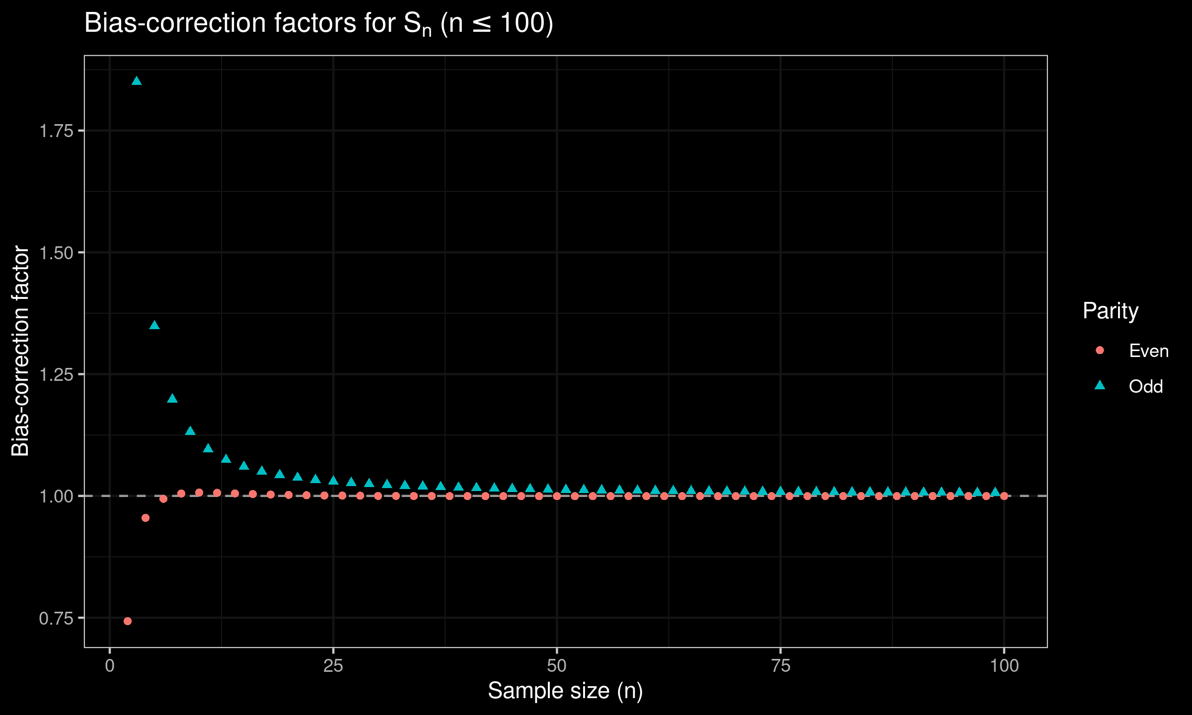
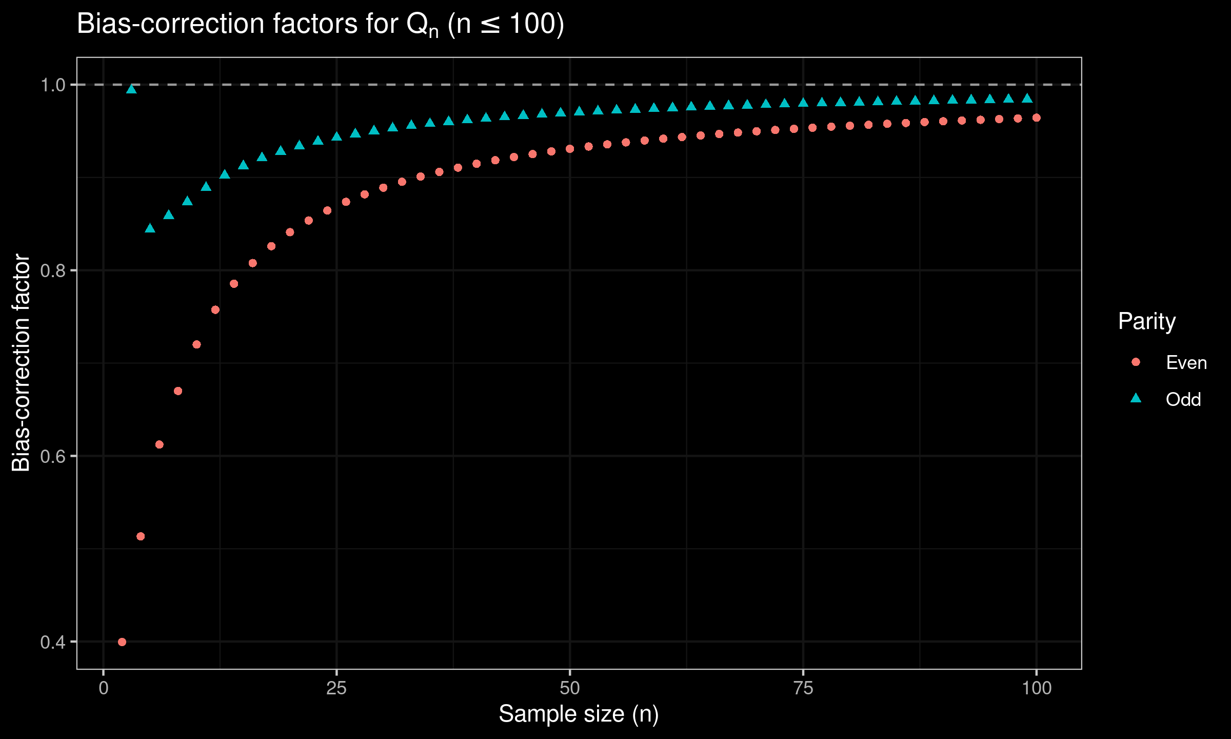
In order to obtain refined values of the bias-correction factors, we perform an extensive Monte-Carlo simulations. Here are the raw results for $n \leq 100$:

n	$c_n$	$d_n$
2	0.74303	0.39954
3	1.84983	0.99386
4	0.95505	0.51333
5	1.34857	0.84412
6	0.99413	0.61224
7	1.19832	0.85886
8	1.00496	0.67000
9	1.13178	0.87359
10	1.00689	0.72007
11	1.09592	0.88902
12	1.00635	0.75748
13	1.07423	0.90232
14	1.00513	0.78551
15	1.06006	0.91248
16	1.00384	0.80779
17	1.05006	0.92106
18	1.00281	0.82600
19	1.04297	0.92793
20	1.00219	0.84105
21	1.03738	0.93380
22	1.00139	0.85367
23	1.03311	0.93894
24	1.00091	0.86441
25	1.02969	0.94303
26	1.00066	0.87372
27	1.02686	0.94680
28	1.00045	0.88186
29	1.02449	0.95009
30	1.00005	0.88901
31	1.02260	0.95304
32	0.99995	0.89531
33	1.02087	0.95566
34	0.99974	0.90099
35	1.01950	0.95789
36	0.99978	0.90600
37	1.01830	0.96004
38	0.99960	0.91061
39	1.01717	0.96192
40	0.99969	0.91480
41	1.01619	0.96361
42	0.99960	0.91852
43	1.01538	0.96522
44	0.99955	0.92200
45	1.01460	0.96668
46	0.99960	0.92515
47	1.01391	0.96802
48	0.99948	0.92809
49	1.01324	0.96923
50	0.99953	0.93085
51	1.01264	0.97040
52	0.99954	0.93334
53	1.01228	0.97147
54	0.99949	0.93566
55	1.01175	0.97237
56	0.99950	0.93781
57	1.01127	0.97328
58	0.99955	0.93985
59	1.01090	0.97421
60	0.99959	0.94180
61	1.01054	0.97496
62	0.99954	0.94355
63	1.01023	0.97573
64	0.99963	0.94525
65	1.00988	0.97648
66	0.99968	0.94687
67	1.00951	0.97710
68	0.99959	0.94837
69	1.00923	0.97773
70	0.99966	0.94978
71	1.00902	0.97837
72	0.99965	0.95112
73	1.00877	0.97891
74	0.99964	0.95235
75	1.00851	0.97944
76	0.99966	0.95359
77	1.00835	0.97999
78	0.99968	0.95472
79	1.00810	0.98049
80	0.99966	0.95579
81	1.00790	0.98090
82	0.99970	0.95677
83	1.00765	0.98138
84	0.99970	0.95781
85	1.00762	0.98179
86	0.99968	0.95871
87	1.00740	0.98216
88	0.99972	0.95967
89	1.00723	0.98255
90	0.99973	0.96051
91	1.00705	0.98295
92	0.99974	0.96139
93	1.00689	0.98329
94	0.99974	0.96212
95	1.00674	0.98363
96	0.99978	0.96294
97	1.00661	0.98399
98	0.99973	0.96364
99	1.00650	0.98430
100	0.99982	0.96438

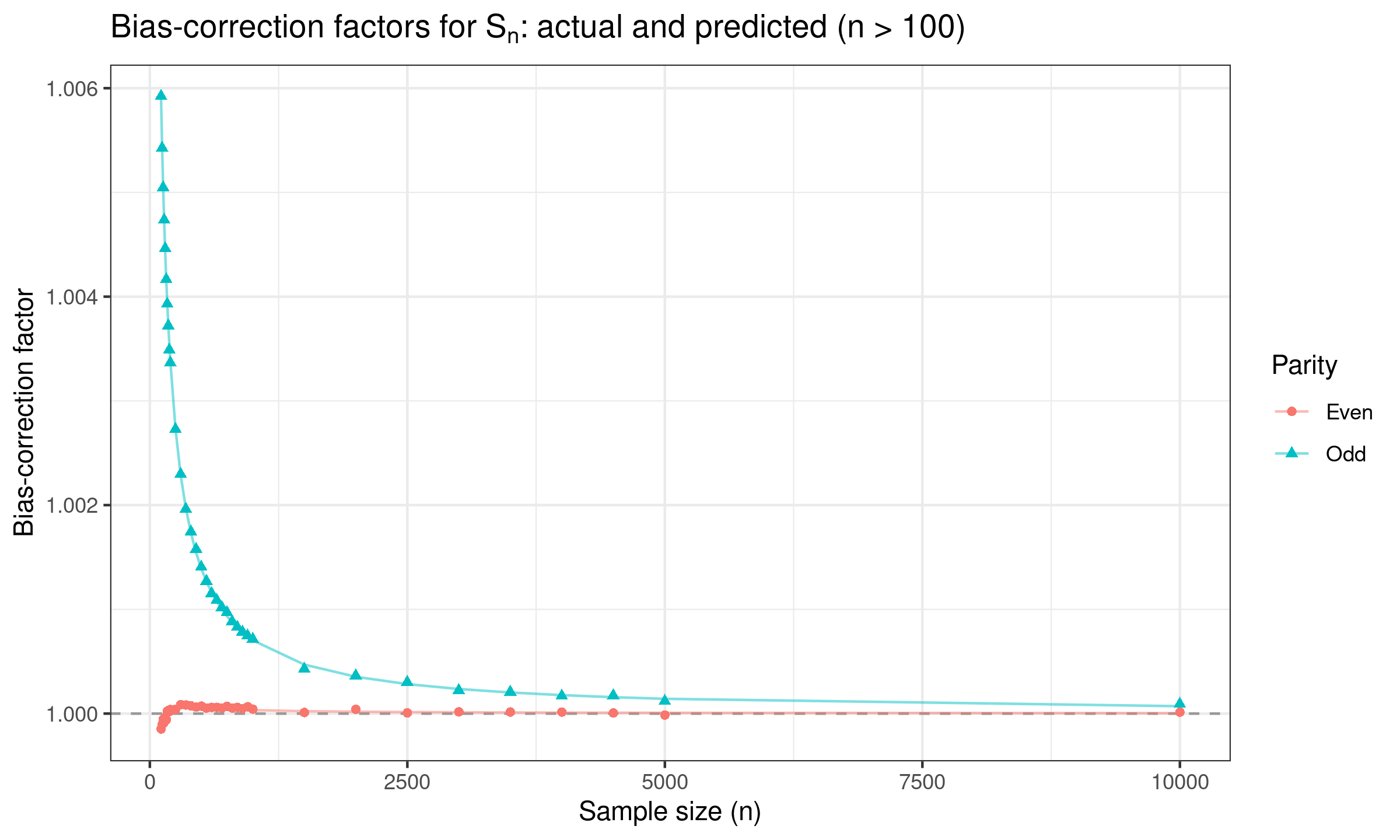
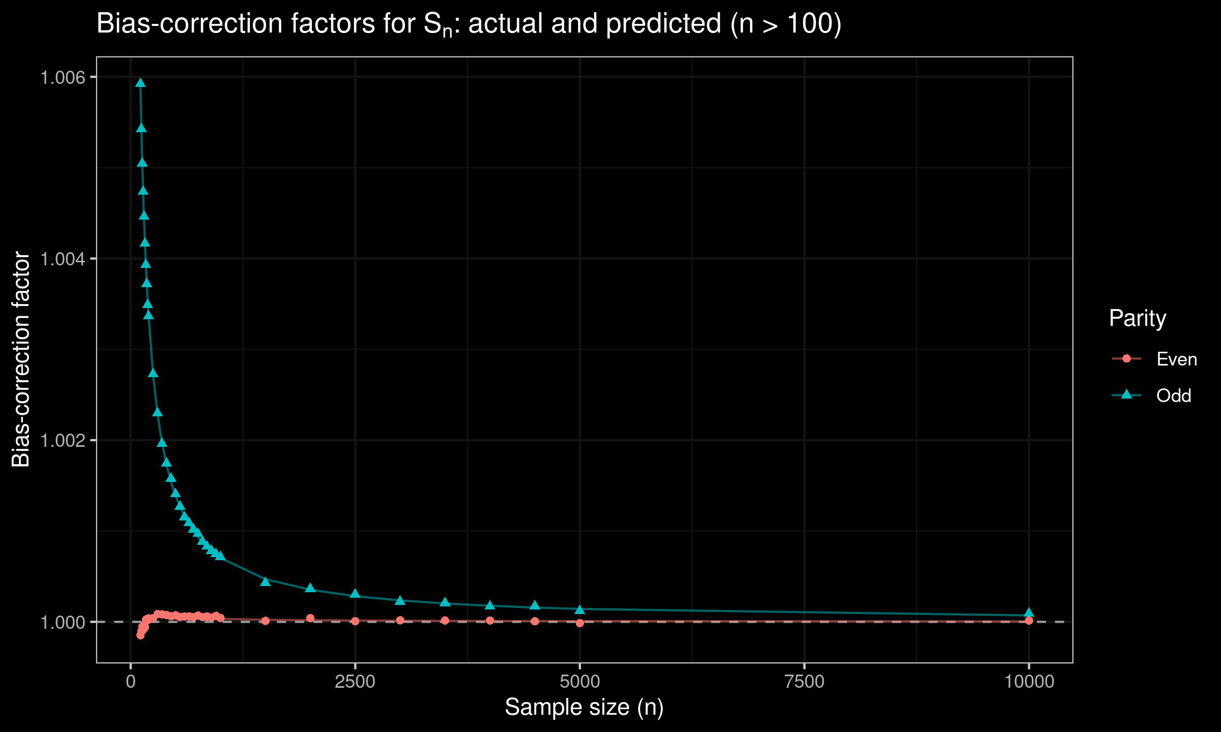
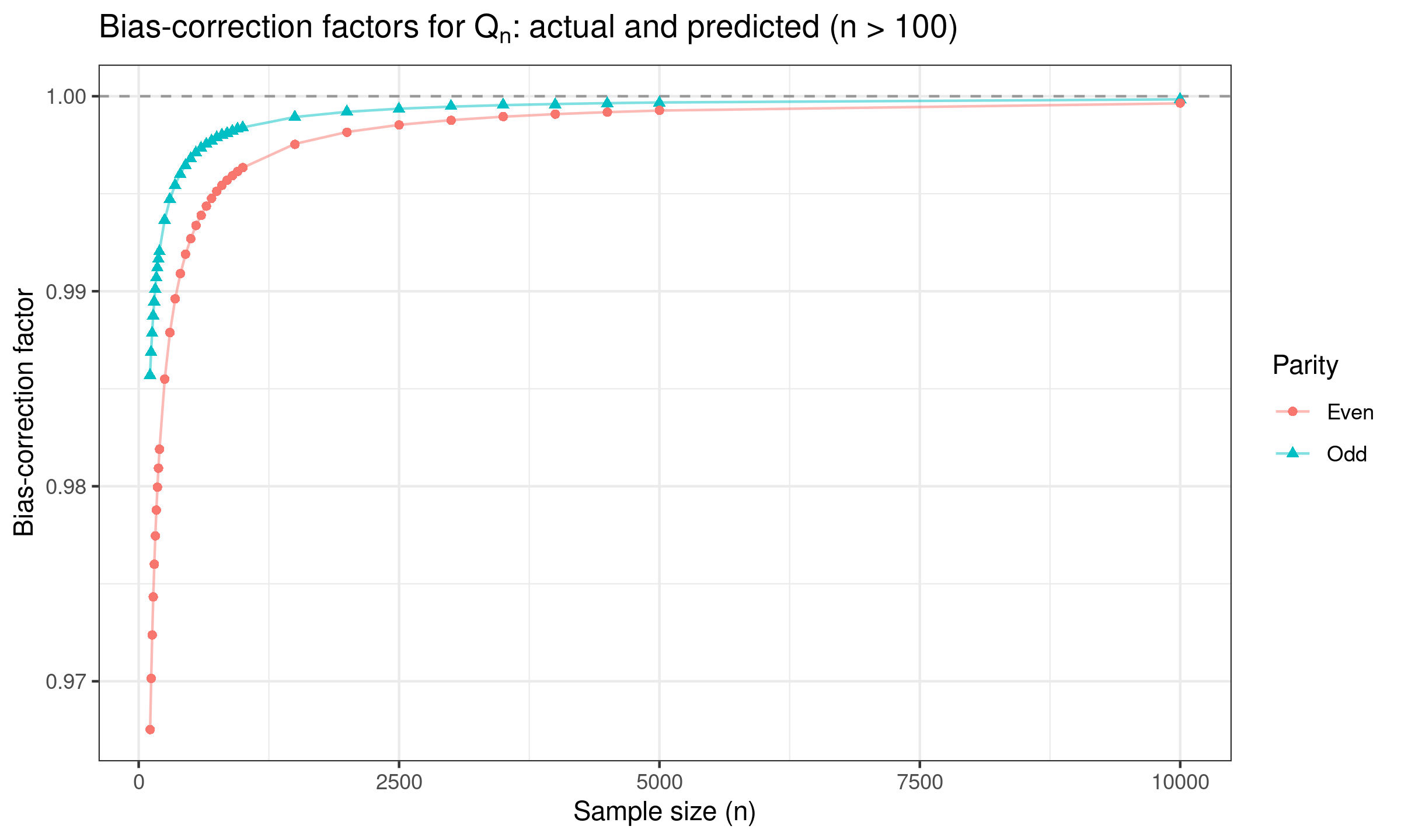
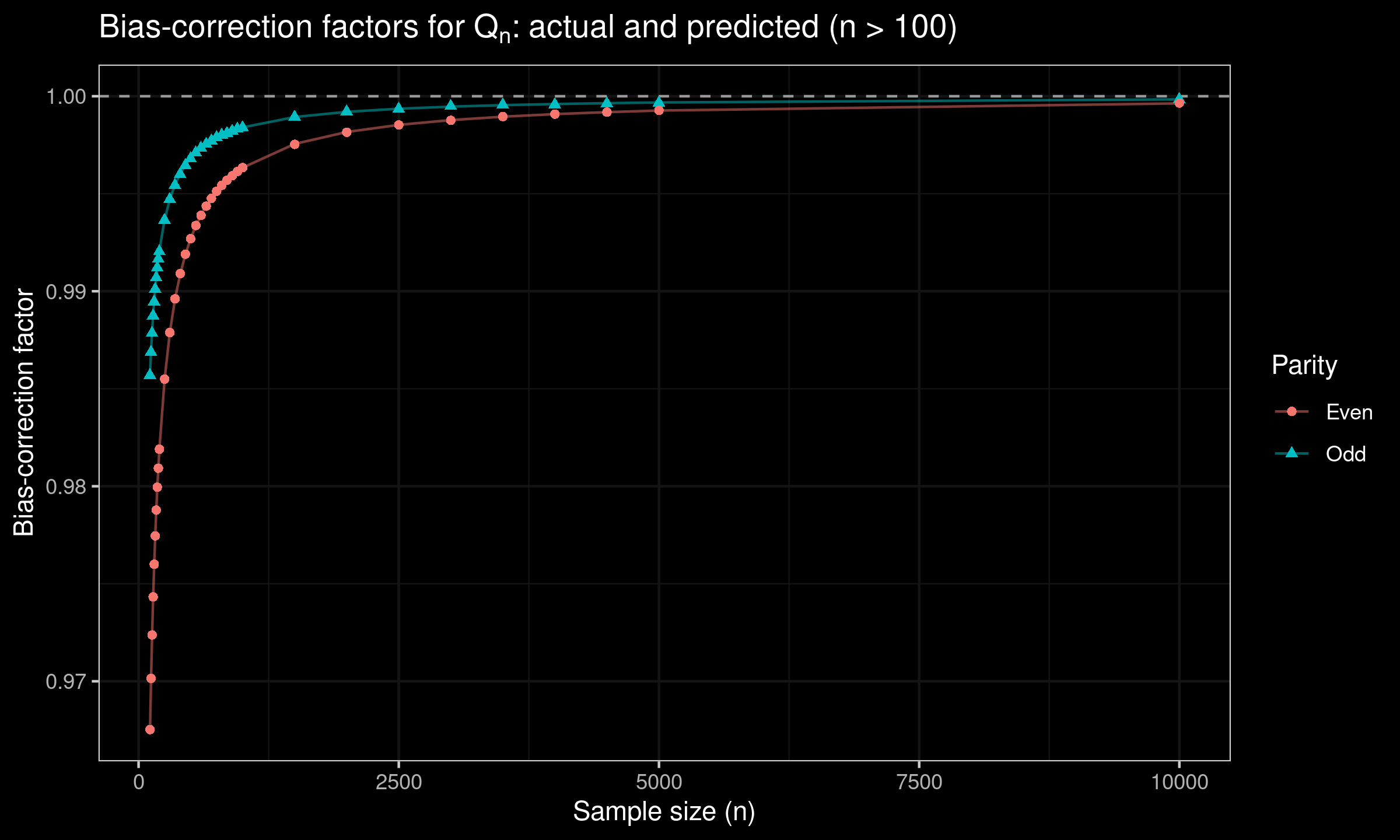
For $n > 100$, we suggest using the following prediction equations:

$$ c_n = 1 + 0.7096 n^{-1} - 7.3604 n^{-2}, \quad \textrm{for odd}\; n, $$$$ c_n = 1 + 0.0391 n^{-1} - 6.1719 n^{-2}, \quad \textrm{for even}\; n, $$$$ d_n = 1 - 1.6022 n^{-1} + 4.7453 n^{-2}, \quad \textrm{for odd}\; n, $$$$ d_n = 1 -3.6741 n^{-1} + 11.1030 n^{-2}, \quad \textrm{for even}\; n. $$

Here are the corresponding plots:

References

• [Croux1992]
  Croux, Christophe, and Peter J. Rousseeuw. “Time-Efficient Algorithms for Two Highly Robust Estimators of Scale.” In Computational Statistics, edited by Yadolah Dodge and Joe Whittaker, 411–28. Heidelberg: Physica-Verlag HD, 1992.
  https://doi.org/10.1007/978-3-662-26811-7_58.
• [Rousseeuw1993]
  Rousseeuw, Peter J., and Christophe Croux. “Alternatives to the Median Absolute Deviation.” Journal of the American Statistical Association 88, no. 424 (December 1, 1993): 1273–83.
  https://doi.org/10.1080/01621459.1993.10476408.