Shift function vs. shift distribution
Let’s say we have two distributions $X$ and $Y$, and we want to express the “absolute difference” between them. This abstract term could be expressed in various ways. My favorite approach is to build the Doksum’s shift function. In order to do this, for each quantile $p$, we should calculate $Q_Y(p)-Q_X(p)$ where $Q$ is the quantile function. However, some people prefer using the shift distribution $Y-X$. While both approaches may provide similar results for narrow non-overlapping distributions, they are not equivalent in the general case. In this post, we briefly consider examples of both approaches.
Equal normal distributions
Let’s start with a simple case when both $X$ and $Y$ are the standard normal distributions:
$X=Y=\mathcal{N}(0,1)$.
Since distributions are equal, they have equal quantile functions: $Q_X=Q_Y$.
Thus $Q_Y(p)-Q_X(p)$ is zero for all $p$ values.
Here is the corresponding Doksum’s shift function
(see Empirical Probability Plots and Statistical Inference for Nonlinear Models in the Two-Sample Case
By Kjell Doksum
·
1974doksum1974):
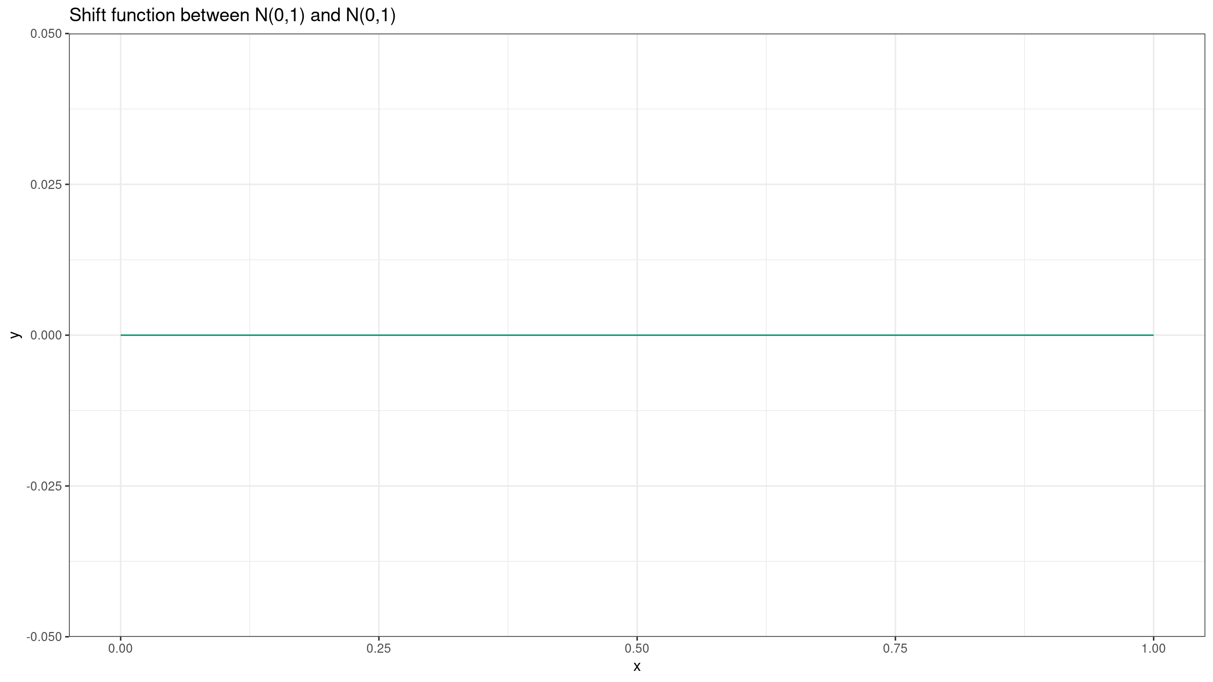
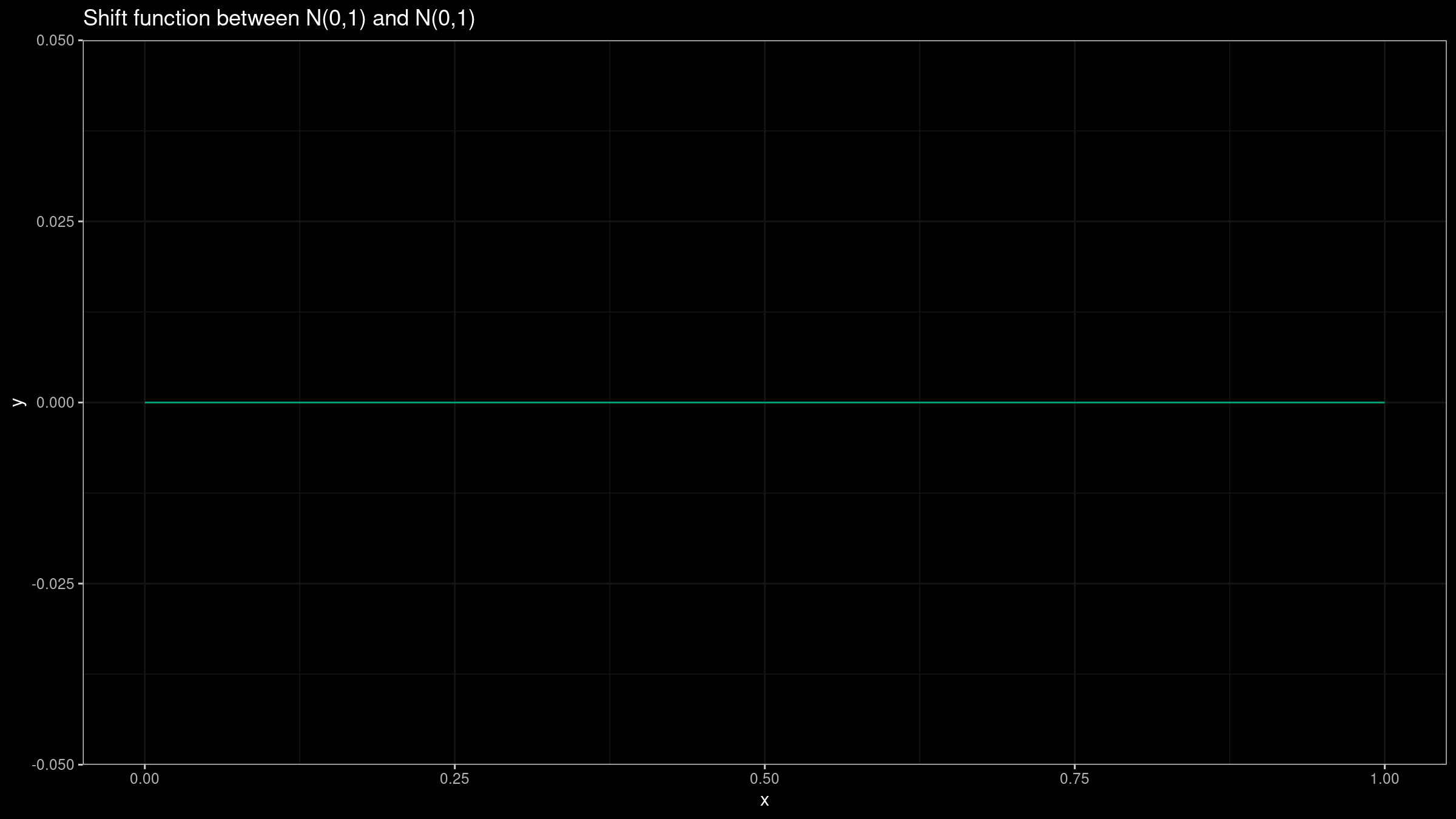
Such a shift function tells us that there is no difference between $X$ and $Y$. If we want to build the shift function for samples, we should just estimate quantiles for both samples. As a robust and statistically efficient quantile estimator we can use the trimmed Harrell-Davis quantile estimator (see [Akinshin2021]).
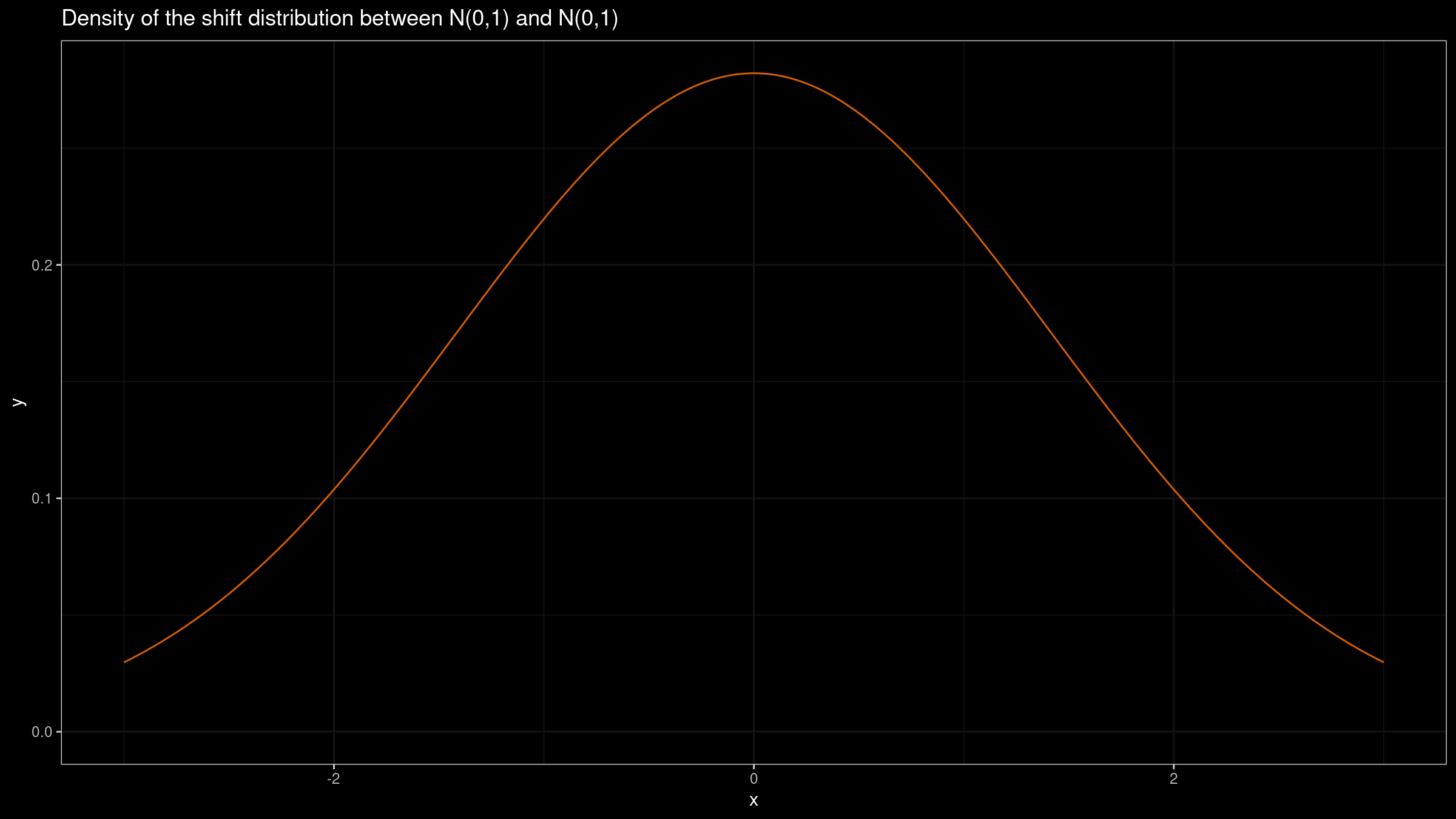
We can also build the shift distribution $Y-X$. If we have two samples of equal size $x=\{x_1, x_2, \ldots, x_n \}$ and $y=\{y_1, y_2, \ldots, y_n\}$, we can estimate the shift distribution based on a sample pairwise differences: $\{y_1-x_1, y_2-x_2, \ldots, y_n-x_n\}$. This distribution provides insights about the difference of two random elements from $X$ and $Y$, but it doesn’t provide a clear picture of the actual difference between distributions. The sum of two normal distributions is also a normal distribution: $\mathcal{N}(\mu_X, \sigma^2_X)+\mathcal{N}(\mu_Y, \sigma^2_Y)=\mathcal{N}(\mu_X+\mu_Y, \sigma^2_X+\sigma^2_Y)$. Thus, $Y-X = \mathcal{N}(0, 1) + (-\mathcal{N}(0, 1)) = \mathcal{N}(0, 1) + \mathcal{N}(0, 1) = \mathcal{N}(0, 2)$. Here is the corresponding plot:

Different normal distributions (small difference)
Now let’s consider two different normal distributions: $X=\mathcal{N}(0,1)$, $Y=\mathcal{N}(2,1)$. It’s easy to see that the shift function is defined as $Q_Y(p)-Q_X(p)=2$ for all $p$ values:

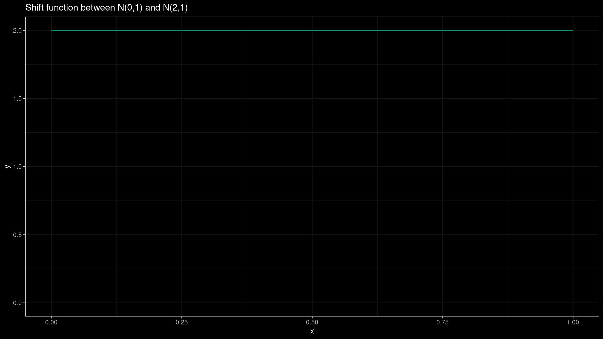
Such a plot provides a clear insight about the actual difference between $X$ and $Y$.
Now let’s build the shift distribution: $Y-X = \mathcal{N}(2, 1) + (-\mathcal{N}(0, 1)) = \mathcal{N}(2, 1) + \mathcal{N}(0, 1) = \mathcal{N}(2, 2)$:
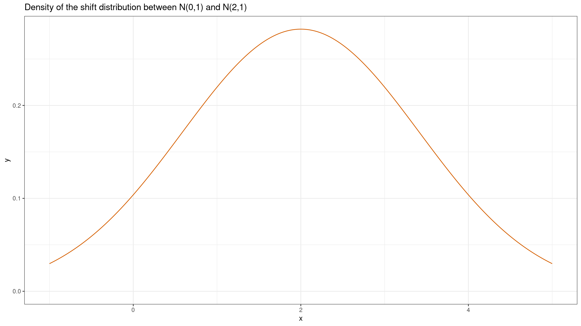

Although this plot could provide some valuable insights (e.g., it’s quite possible to get a negative value of $Y_1-X_1$), it doesn’t actually describe the actual difference between distributions.
Different normal distributions (big difference)
Let’s repeat the experiment for $X=\mathcal{N}(0,1)$, $Y=\mathcal{N}(100,1)$:
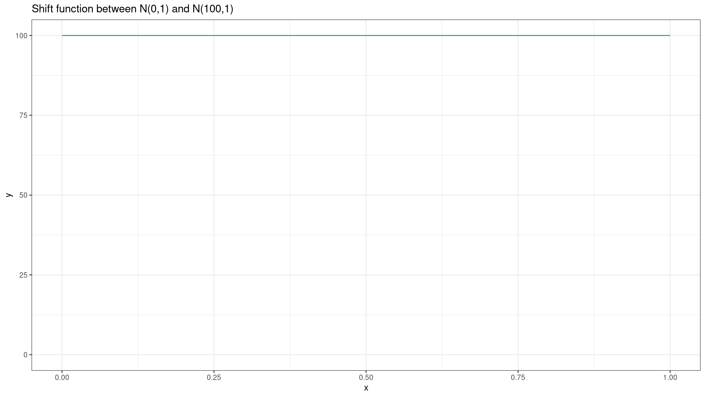
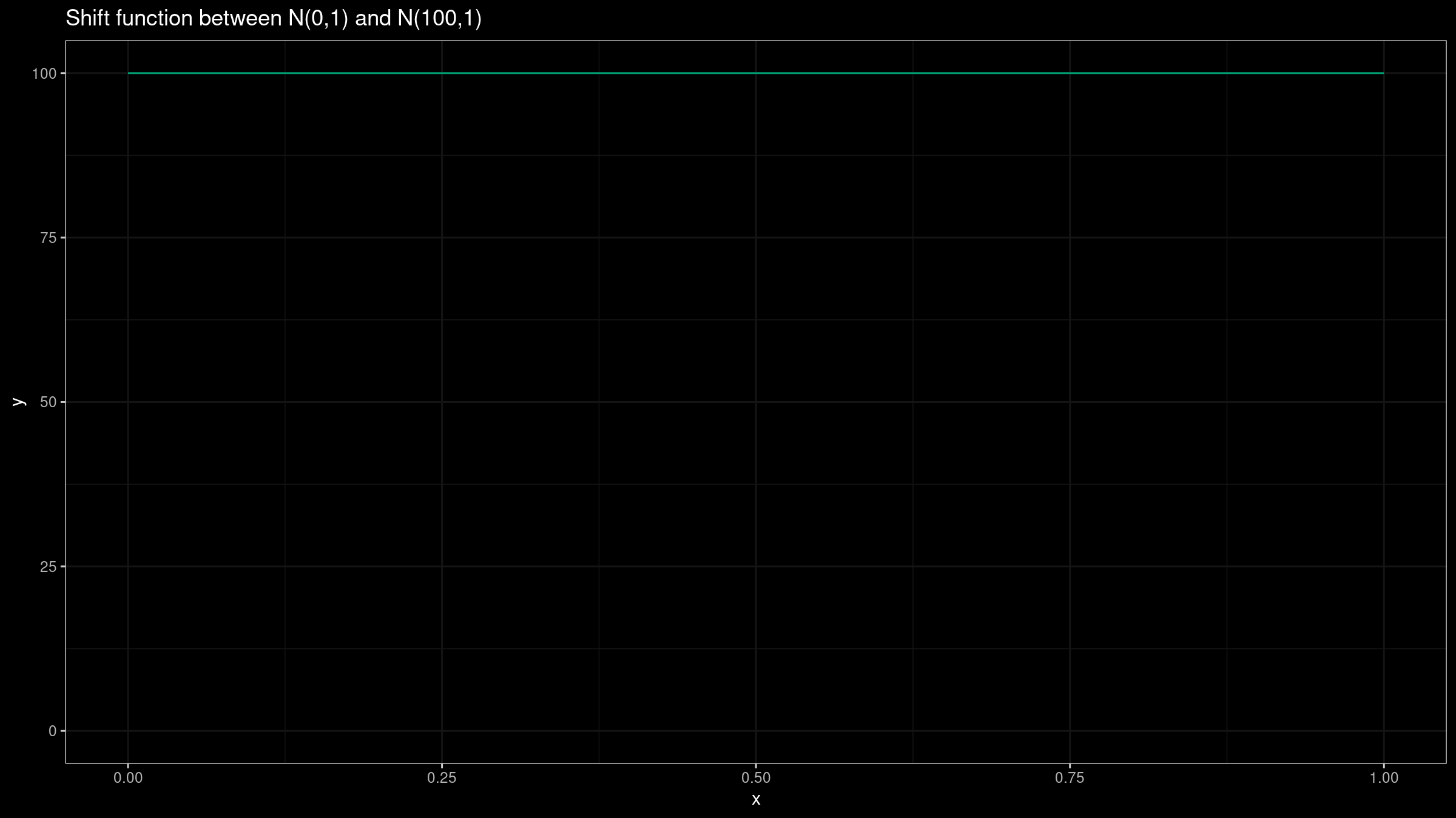
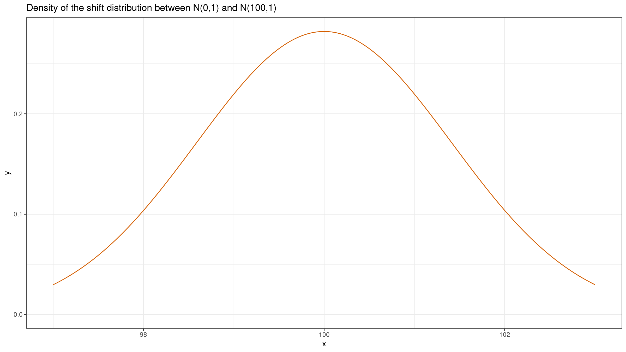
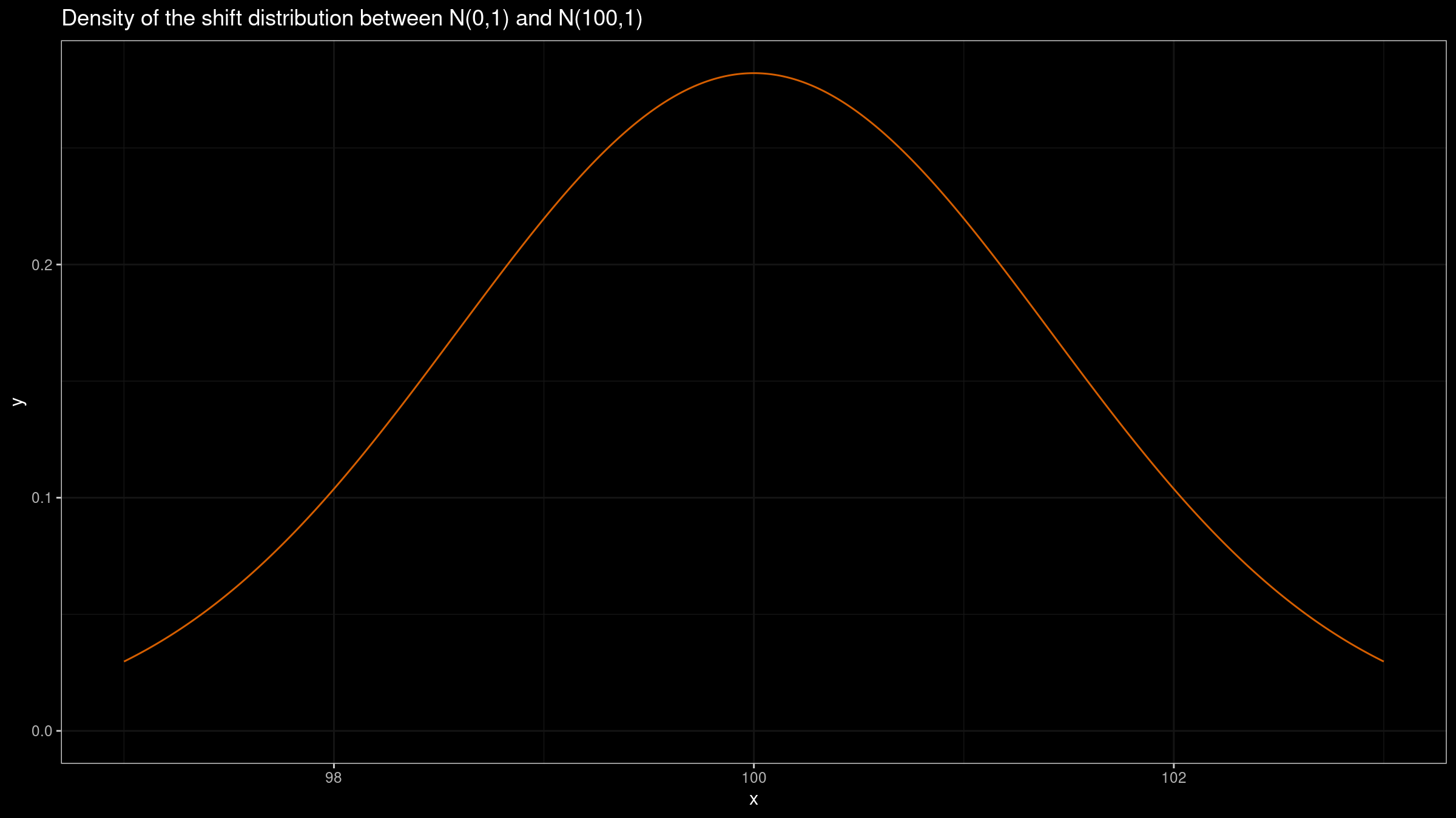
In this case, we could get the same insight from both plots: the difference between $X$ and $Y$ is about $100$. If we build such plots based on small samples, they could provide similar ranges because of the noise. However, we should keep in mind that this trick doesn’t work in the general case.
Uniform distributions
Lastly, let’s build both plots for two uniform distributions: $X=\mathcal{U}(-1,1)$, $Y=\mathcal{U}(0,1)$.
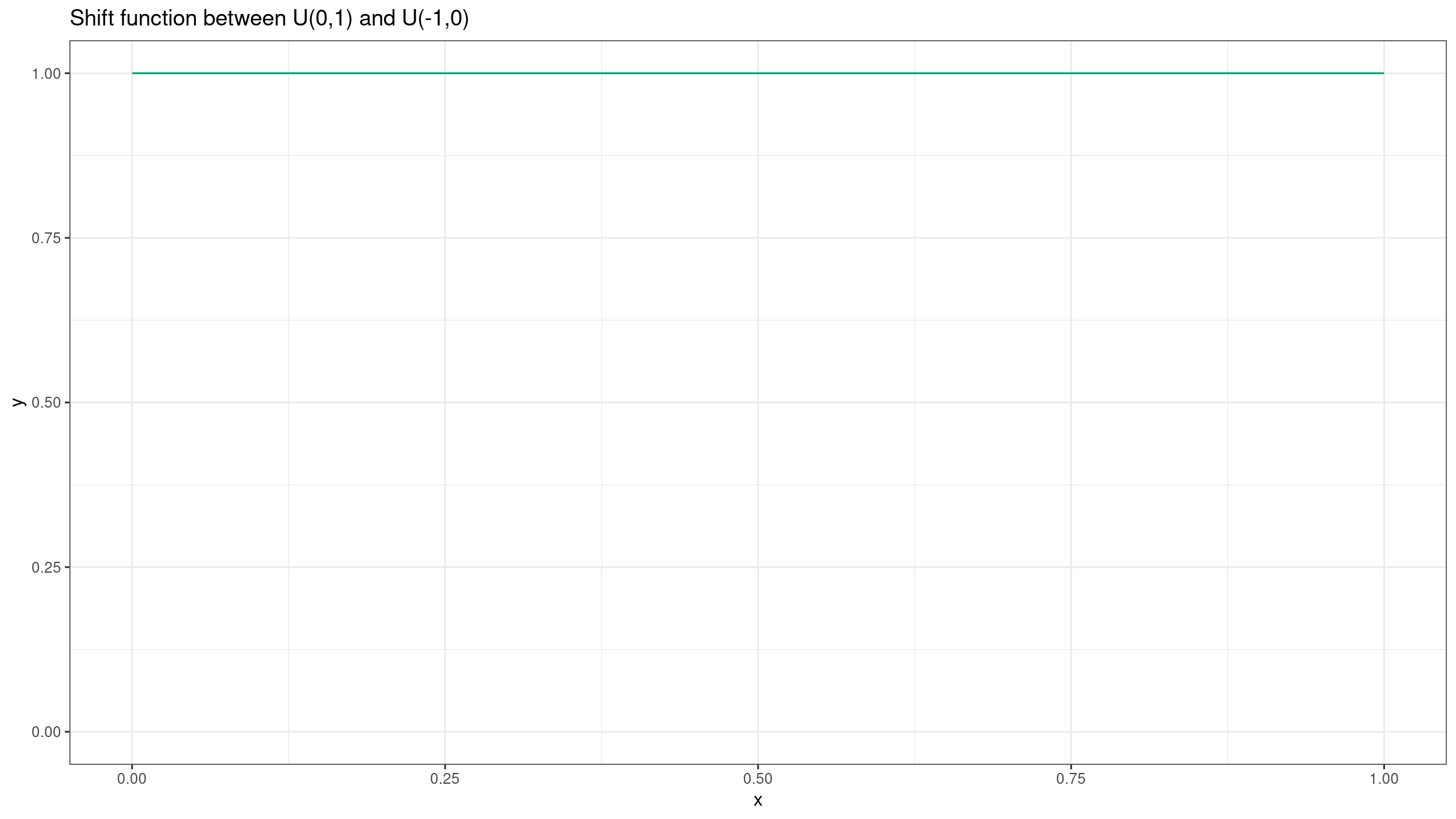

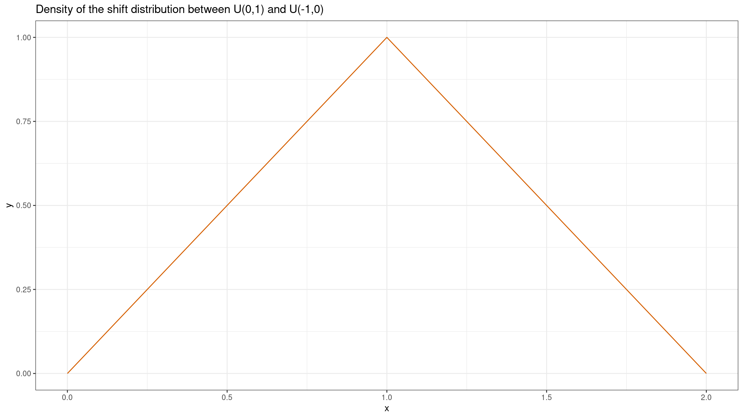
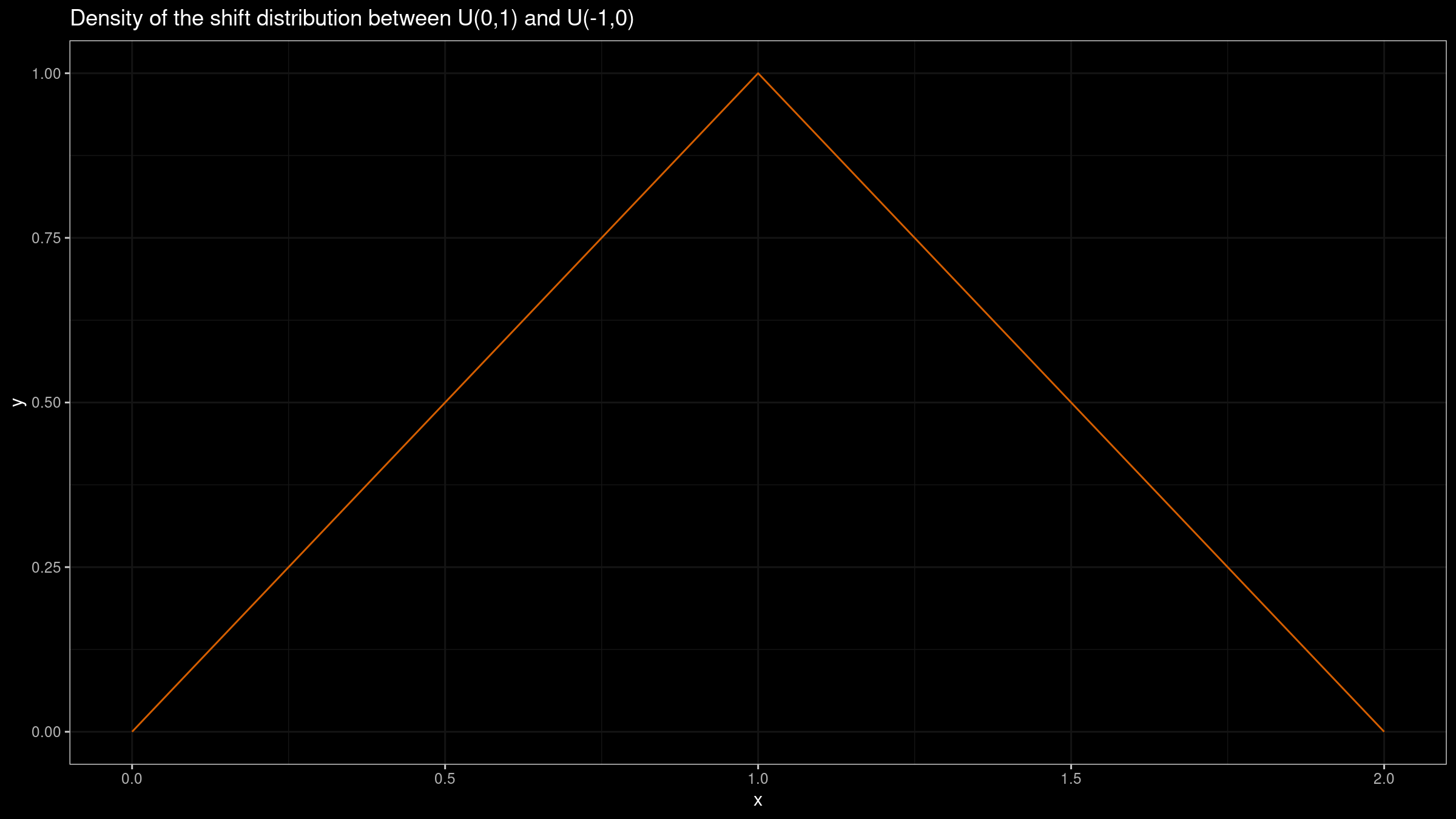
While the shift function is still a constant ($Q_Y(p)-Q_X(p)=1$), we have a triangular shift distribution $\textrm{Tri}(0, 2, 1)$.
Conclusion
Both the shift function and the shift distribution may provide useful insights about the properties of the difference between $X$ and $Y$. However, if we want to get the picture about the actual absolute difference between distribution PDFs, the shift function works much better.
References
- [Doksum1974]
Doksum, Kjell. “Empirical probability plots and statistical inference for nonlinear models in the two-sample case.” The annals of statistics (1974): 267-277.
https://doi.org/10.1214/aos/1176342662 - [Akinshin2021]
Andrey Akinshin (2021) Trimmed Harrell-Davis quantile estimator based on the highest density interval of the given width,
arXiv:2111.11776