Standard quantile absolute deviation

The median absolute deviation (MAD) is a popular robust replacement of the standard deviation (StdDev). It’s truly robust: its breakdown point is $50\%$. However, it’s not so efficient when we use it as a consistent estimator for the standard deviation under normality: the asymptotic relative efficiency against StdDev (we call it the Gaussian efficiency) is only about $\approx 37\%$.

In practice, such robustness is not always essential, while we typically want to have the highest possible efficiency. I already described the concept of the quantile absolute deviation which aims to provide a customizable trade-off between robustness and efficiency. In this post, I would like to suggest a new default option for this measure of dispersion called the standard quantile absolute deviation. Its Gaussian efficiency is $\approx 54\%$ while the breakdown point is $\approx 32\%$

Introduction

In the context of this post, we consider the quantile absolute deviation ($\operatorname{QAD}$) around the median:

$$ \newcommand{MAD}{\operatorname{MAD}} \newcommand{QAD}{\operatorname{QAD}} \newcommand{SQAD}{\operatorname{SQAD}} \newcommand{Q}{\operatorname{Q}} \newcommand{SD}{\operatorname{SD}} \newcommand{QHF}{\operatorname{Q}_{\operatorname{HF7}}} \newcommand{QHD}{\operatorname{Q}_{\operatorname{HD}}} \newcommand{QTHD}{\operatorname{Q}_{\operatorname{THD-SQRT}}} \newcommand{erf}{\operatorname{erf}} \newcommand{erfinv}{\operatorname{erf}^{-1}} \newcommand{E}{\mathbb{E}} \newcommand{V}{\mathbb{V}} \QAD(X, p) = \Q(|X - \Q(X, 0.5)|, p), $$

where $Q$ is a quantile estimator, X is a sample of i.i.d. random variables $X = \{ X_1, X_2, \ldots, X_n \}$.

Obviously, the median absolute deviation is a special case of $\operatorname{QAD}$:

$$ \MAD(X) = \Q(|X - \Q(X, 0.5)|, 0.5) = \QAD(X, 0.5). $$

As for $\Q$, we consider the traditional quantile estimator $\QHF$ (Type 7 in the Hyndman-Fan taxonomy, see hyndman1996).

Efficiency vs. robustness

The classic standard equation estimator provides great Gaussian efficiency for the standard deviation, but it is not robust (the breakdown point is 0.0). The median absolute deviation provides poor Gaussian efficiency, but it is highly robust (the breakdown point is 0.5). When we choose an estimator, we always have to deal with a trade-off between efficiency and robustness. Finding the right balance can be a challenging task.

It is said that $\MAD$ has the highest possible breakdown point for a scale estimator. Though, we have a theoretical option to build a scale estimator with a higher breakdown point (e.g., $\QAD(X, 0.25)$). However, such an estimator would not make much sense. Indeed, if more than 50% of the sample elements are corrupted by outliers, these outliers become the major part of the distribution. If these outliers are non-representative (obtained due to measurements error or other technical mistakes; gross errors), we should completely ignore them or reconsider the way we collect the data. Moreover, if the median itself is corrupted, estimating the deviation around the median is meaningless. If these outliers are representative (actually describe the true nature of the underlying model), we should treat them as a part of the distribution.

While 0.5 is the highest breakdown point for a scale estimator, it is not necessarily the optimal one. Let us consider a situation when 49% of a sample is contaminated by outliers. The $\MAD$ could handle such a situation and provide a non-corrupted estimation. But do we really want to use $\MAD$ in such a situation? If 49% of sample elements are outliers, do we really want to consider them as outliers? At some moment, it makes sense to consider them as an essential part of a distribution. Probably the distribution is multimodal, and it makes sense to consider each mode separately. Anyway, a single $\MAD$ value can be quite misleading in such a situation.

Now let us say that we have learned to detect samples with a significant number of outliers to analyze them using a dedicated approach. In this case, we do not really need the 0.5 breakdown point. This means that we can trade some robustness for statistical efficiency. The next reasonable question is how to choose the optimal breakdown point.

Choosing the breakdown point

Let us recall the density plot of the normal distribution:

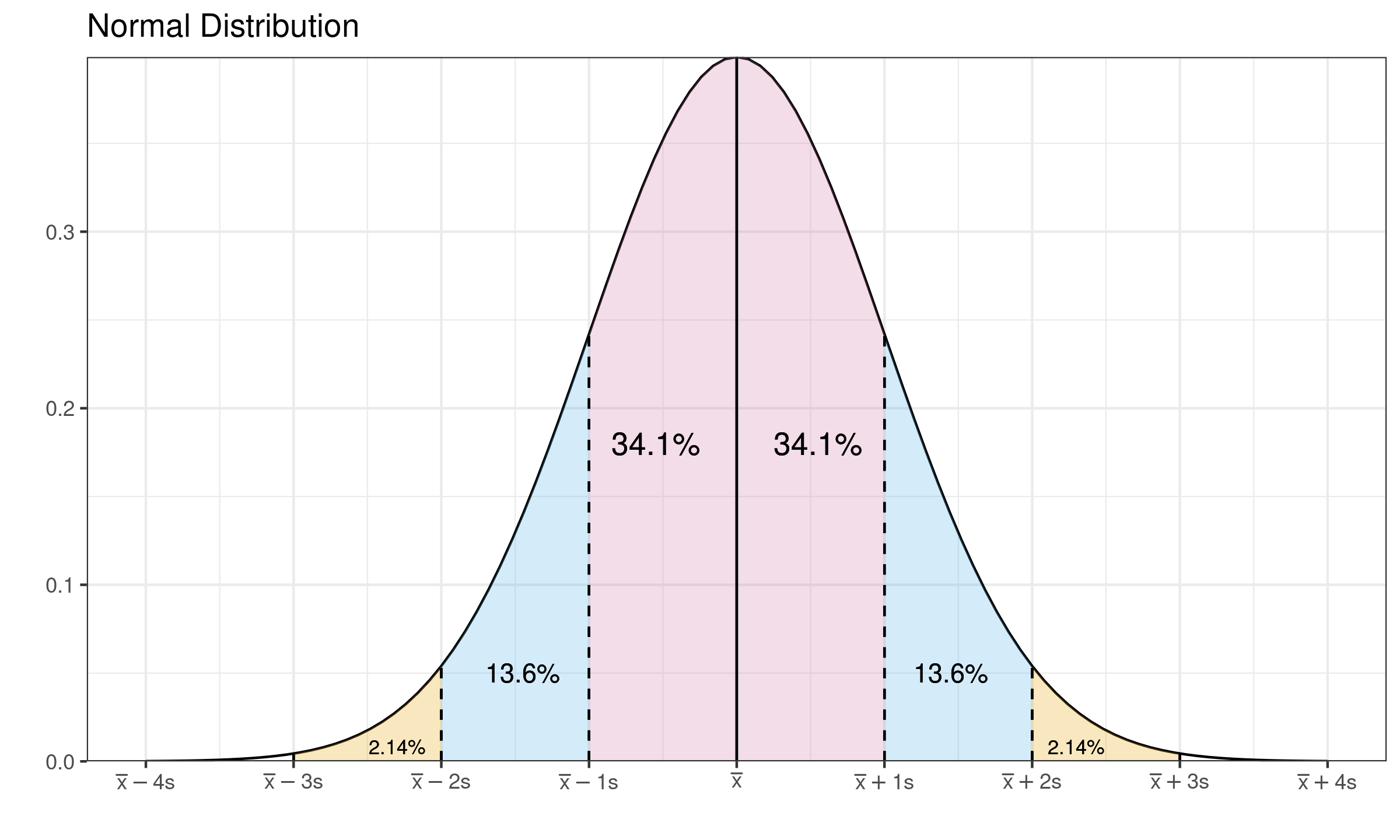
The $\MAD$ and other measures of dispersion are often used as consistency estimators for the standard deviation. The idea is simple: we estimate the $\MAD$, multiply it by a scale constant and get the standard deviation. It works well when the distribution is continuous, light-tailed, unimodal, and with only slight deviations from normality. In this case, we typically assume that the interval $[\mu-\sigma; \mu+\sigma]$ is not so distorted compared to the normal distribution. This assumption is violated if some elements of $[\mu-\sigma; \mu+\sigma]$ are corrupted. Let us consider the “protection” of this interval as a reference condition for choosing the breakdown point. For the normal distribution, $[\mu-\sigma; \mu+\sigma]$ covers exactly $\Phi(1)-\Phi(-1) = 2\Phi(1) - 1 \approx 0.6827 = 68.27\%$ of the distribution. It gives us a breakdown point which is equal to $1 - (\Phi(1)-\Phi(-1)) \approx 0.3173 = 31.73\%$. It could be interpreted as follows: if less than one-third of the distribution is contaminated, we are in the safe zone: the scale estimations are not corrupted. If more than one-third of the distribution is contaminated, we should split the distribution into several modes and analyze each mode independently. The breakdown point of $37.73\%$ looks like an admissible value.

The standard quantile absolute deviation

Since we have the desired asymptotic breakdown point, we can define the corresponding measure of scale using $\QAD$. Let us denote it by the standard quantile absolute deviation or $\SQAD$. Asymptotically, it can be defined as follows:

$$ \SQAD(X) = \QAD(X, 2\Phi(1) - 1). $$

There is no need to introduce a scale constant: the asymptotic expected value of $\SQAD$ for the normal distribution is 1 (since the sample quantile are Fisher-consistent for the distribution quantiles when $f(p)>0$ (see Theorem 8.5.1 in arnold2008), $\SQAD$ is Fisher-consistent for the standard deviation):

$$ \E[\SQAD(X)] = \E[\QAD(X, 2\Phi(1) - 1)] = \E[Q(|X|, 2\Phi(1) - 1)] = 1. $$

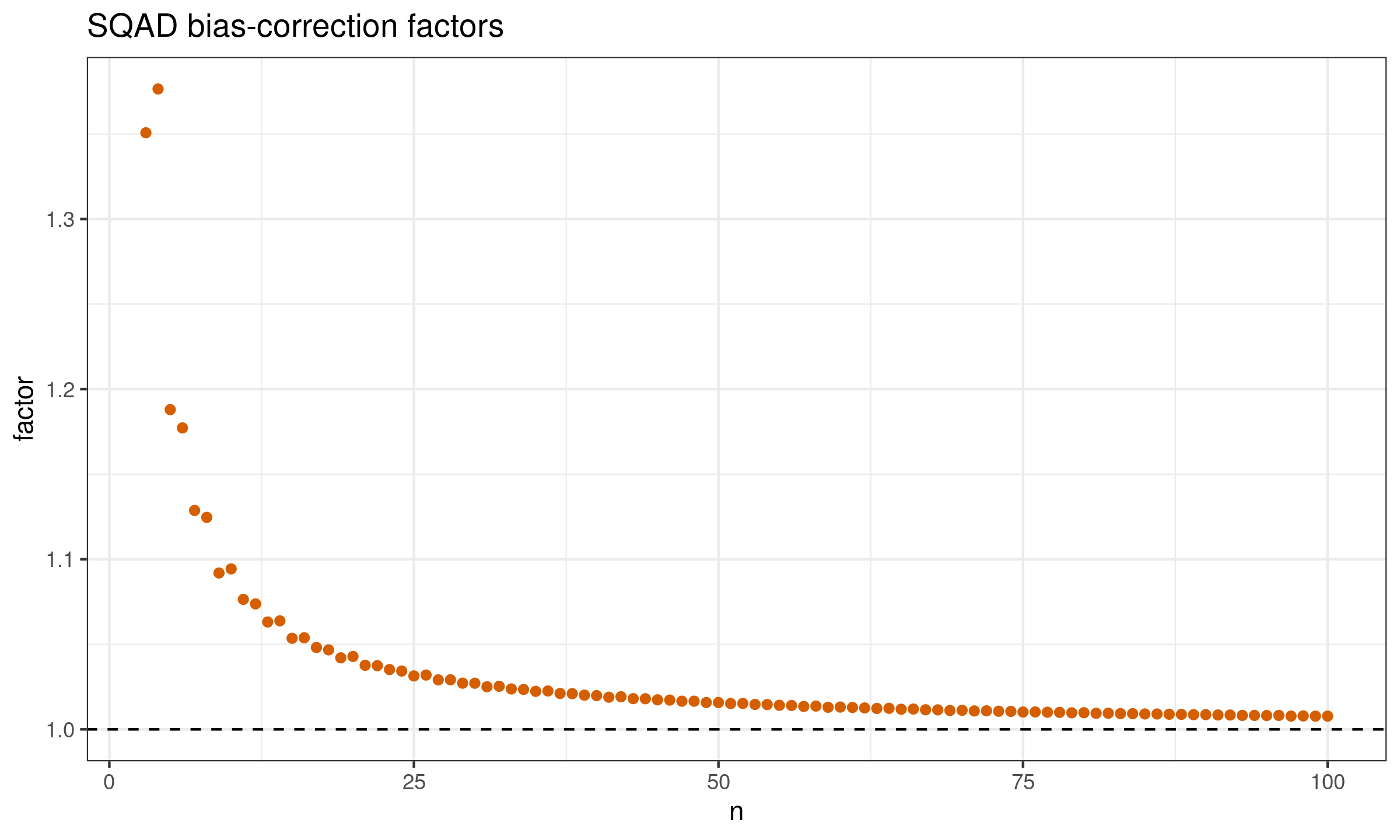
If we want to make $\SQAD$ an unbiased estimator for $\SD$ under normality, we have to introduce the bias-correction factor $C_n$:

$$ \SQAD_n(X) = C_n \cdot \QAD(X, 2\Phi(1) - 1). $$

The factor values can be easily obtained using Monte-Carlo simulations. Here is the plot with these values for $n \leq 100$:

And here are the raw factor values:

n	factor
3	1.35070
4	1.37644
5	1.18794
6	1.17720
7	1.12869
8	1.12460
9	1.09191
10	1.09434
11	1.07640
12	1.07376
13	1.06312
14	1.06379
15	1.05354
16	1.05383
17	1.04811
18	1.04673
19	1.04203
20	1.04285
21	1.03765
22	1.03745
23	1.03516
24	1.03428
25	1.03139
26	1.03192
27	1.02910
28	1.02915
29	1.02715
30	1.02712
31	1.02504
32	1.02533
33	1.02376
34	1.02346
35	1.02234
36	1.02257
37	1.02110
38	1.02097
39	1.02011
40	1.01985
41	1.01890
42	1.01917
43	1.01806
44	1.01800
45	1.01735
46	1.01722
47	1.01654
48	1.01655
49	1.01577
50	1.01577
51	1.01518
52	1.01524
53	1.01466
54	1.01458
55	1.01413
56	1.01404
57	1.01347
58	1.01369
59	1.01299
60	1.01310
61	1.01286
62	1.01258
63	1.01230
64	1.01237
65	1.01183
66	1.01194
67	1.01151
68	1.01145
69	1.01109
70	1.01120
71	1.01082
72	1.01089
73	1.01065
74	1.01056
75	1.01019
76	1.01023
77	1.01006
78	1.00999
79	1.00973
80	1.00977
81	1.00945
82	1.00949
83	1.00926
84	1.00923
85	1.00905
86	1.00903
87	1.00888
88	1.00879
89	1.00862
90	1.00864
91	1.00845
92	1.00843
93	1.00819
94	1.00821
95	1.00813
96	1.00820
97	1.00780
98	1.00789
99	1.00776
100	1.00778
109	1.00700
110	1.00698
119	1.00643
120	1.00642
129	1.00585
130	1.00597
139	1.00550
140	1.00557
149	1.00516
150	1.00514
159	1.00484
160	1.00479
169	1.00452
170	1.00460
179	1.00429
180	1.00426
189	1.00401
190	1.00406
199	1.00378
200	1.00381
249	1.00307
250	1.00307
299	1.00258
300	1.00259
349	1.00219
350	1.00219
399	1.00192
400	1.00190
449	1.00173
450	1.00168
499	1.00151
500	1.00152
600	1.00126
700	1.00109
800	1.00094
900	1.00086
1000	1.00076
1500	1.00050
2000	1.00038
3000	1.00026

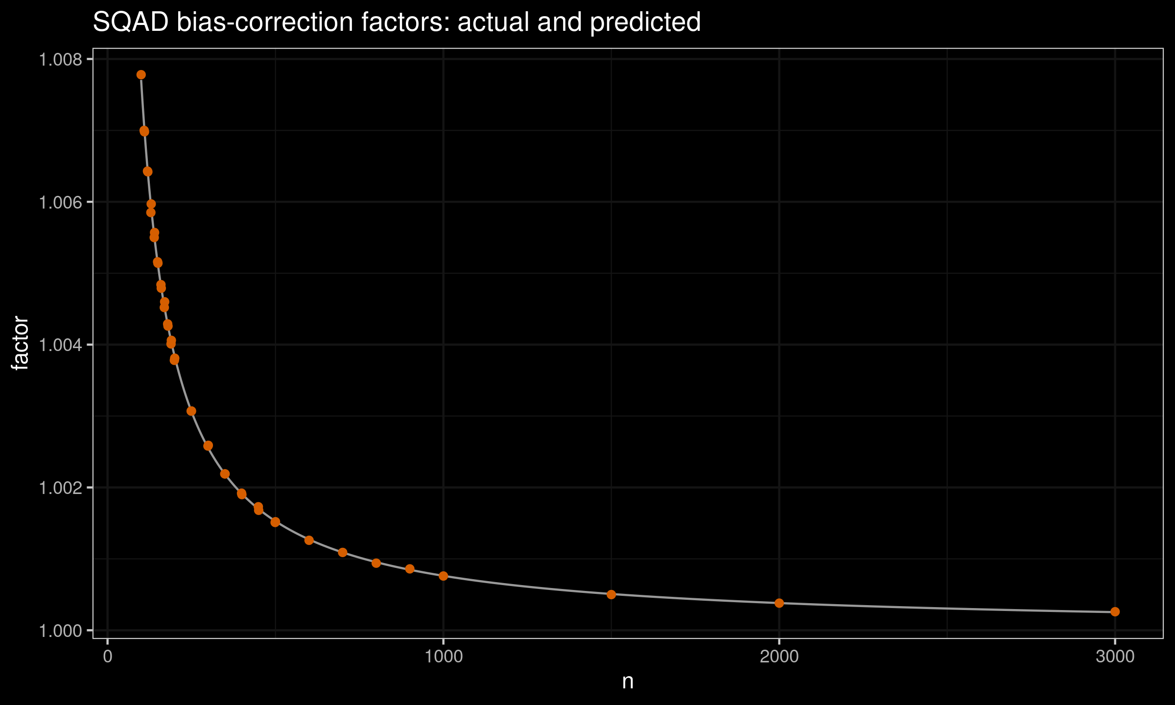
For $n>100$, we can use the following prediction equation (obtained using least squares):

$$ C_n = 1 + 0.762 n +0.868 n^2. $$

This equation perfectly matches the existing estimations:

The statistical efficiency of SQAD and MAD

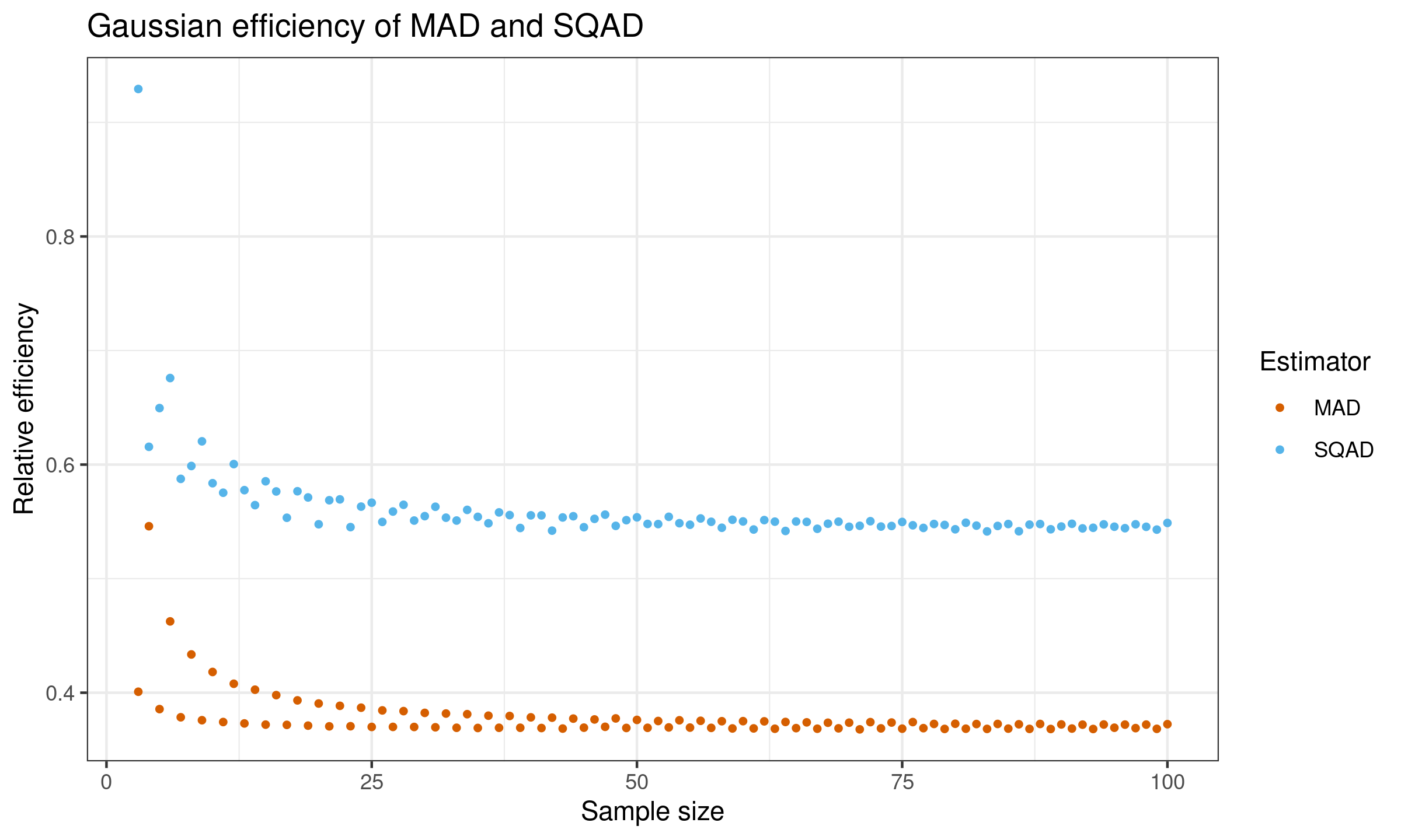
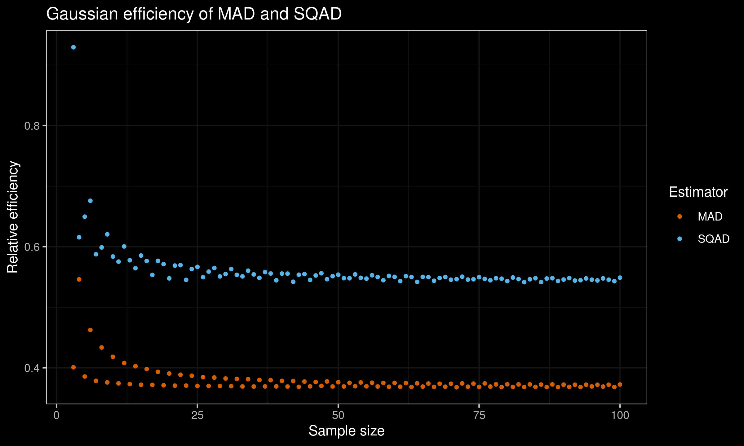
We perform one more simulation study to evaluate the Gaussian efficiency of $\SQAD$ and $\MAD$. As for the baseline, we consider the unbiased standard deviation $\SD_n$:

$$ \SD_n(X) = \sqrt{\frac{1}{n} \sum_{i=1}^n (X_i - \bar{X})^2} \bigg/ c_4(n), \quad c_4(n) = \sqrt{\frac{2}{n-1}}\frac{\Gamma(\frac{n}{2})}{\Gamma(\frac{n-1}{2})}. $$

The scheme of this simulation is straightforward: for each sample size $n$, we generate multiple random samples of the given size from the standard normal distribution. For an unbiased scale estimator $T_n$, we define the Gaussian efficiency as

$$ e(T_n) = \frac{\V[\SD_n]}{\V[T_n]}. $$

Here is the plot of the efficiency values for $n \leq 100$:

And here is the raw efficiency values (including the obtained biases and the standardized variance values):

n	eff.mad	eff.sqad
3	0.40085	0.92931
4	0.54596	0.61559
5	0.38562	0.64954
6	0.46252	0.67588
7	0.37846	0.58748
8	0.43354	0.59877
9	0.37588	0.62040
10	0.41818	0.58368
11	0.37429	0.57532
12	0.40784	0.60043
13	0.37305	0.57759
14	0.40263	0.56445
15	0.37202	0.58536
16	0.39787	0.57645
17	0.37180	0.55338
18	0.39328	0.57663
19	0.37113	0.57120
20	0.39053	0.54768
21	0.37051	0.56875
22	0.38851	0.56950
23	0.37061	0.54519
24	0.38686	0.56315
25	0.36999	0.56659
26	0.38448	0.54974
27	0.37002	0.55883
28	0.38386	0.56476
29	0.36996	0.55093
30	0.38231	0.55479
31	0.36968	0.56303
32	0.38174	0.55344
33	0.36925	0.55094
34	0.38118	0.56029
35	0.36908	0.55418
36	0.37986	0.54853
37	0.36925	0.55809
38	0.37960	0.55573
39	0.36926	0.54442
40	0.37839	0.55552
41	0.36904	0.55548
42	0.37812	0.54209
43	0.36856	0.55365
44	0.37729	0.55472
45	0.36934	0.54509
46	0.37655	0.55243
47	0.37010	0.55612
48	0.37746	0.54628
49	0.36910	0.55126
50	0.37615	0.55376
51	0.36922	0.54797
52	0.37519	0.54783
53	0.36956	0.55422
54	0.37582	0.54860
55	0.36941	0.54726
56	0.37536	0.55278
57	0.36917	0.54985
58	0.37500	0.54461
59	0.36867	0.55163
60	0.37506	0.55015
61	0.36870	0.54308
62	0.37489	0.55133
63	0.36841	0.54997
64	0.37435	0.54182
65	0.36894	0.55011
66	0.37401	0.54976
67	0.36843	0.54372
68	0.37368	0.54816
69	0.36877	0.54995
70	0.37373	0.54550
71	0.36787	0.54635
72	0.37420	0.55036
73	0.36872	0.54567
74	0.37385	0.54617
75	0.36847	0.54970
76	0.37425	0.54679
77	0.36892	0.54448
78	0.37262	0.54791
79	0.36825	0.54709
80	0.37277	0.54329
81	0.36844	0.54902
82	0.37253	0.54649
83	0.36827	0.54142
84	0.37260	0.54621
85	0.36851	0.54788
86	0.37232	0.54154
87	0.36828	0.54736
88	0.37260	0.54789
89	0.36819	0.54330
90	0.37219	0.54570
91	0.36857	0.54809
92	0.37199	0.54407
93	0.36819	0.54459
94	0.37212	0.54758
95	0.36929	0.54554
96	0.37203	0.54423
97	0.36895	0.54764
98	0.37204	0.54546
99	0.36833	0.54300
100	0.37240	0.54883
109	0.36846	0.54636
110	0.37218	0.54689
119	0.36797	0.54649
120	0.37157	0.54510
129	0.36793	0.54593
130	0.37119	0.54175
139	0.36784	0.54373
140	0.37056	0.54266
149	0.36879	0.54139
150	0.37090	0.54441
159	0.36752	0.54201
160	0.37026	0.54493
169	0.36796	0.54429
170	0.37005	0.54434
179	0.36794	0.54417
180	0.37034	0.54388
189	0.36822	0.54427
190	0.36989	0.54206
199	0.36770	0.54290
200	0.36926	0.54206
249	0.36793	0.54262
250	0.36917	0.54152
299	0.36802	0.54363
300	0.36926	0.54122
349	0.36763	0.54216
350	0.36865	0.54212
399	0.36709	0.54143
400	0.36864	0.54230
449	0.36743	0.54104
450	0.36892	0.54312
499	0.36719	0.53987
500	0.36840	0.54189
600	0.36851	0.54134
700	0.36897	0.54134
800	0.36744	0.54142
900	0.36934	0.54187
1000	0.36741	0.53976
1500	0.36821	0.54124
2000	0.36836	0.54144
3000	0.36810	0.54149
10000	0.36782	0.54066
50000	0.36810	0.54080

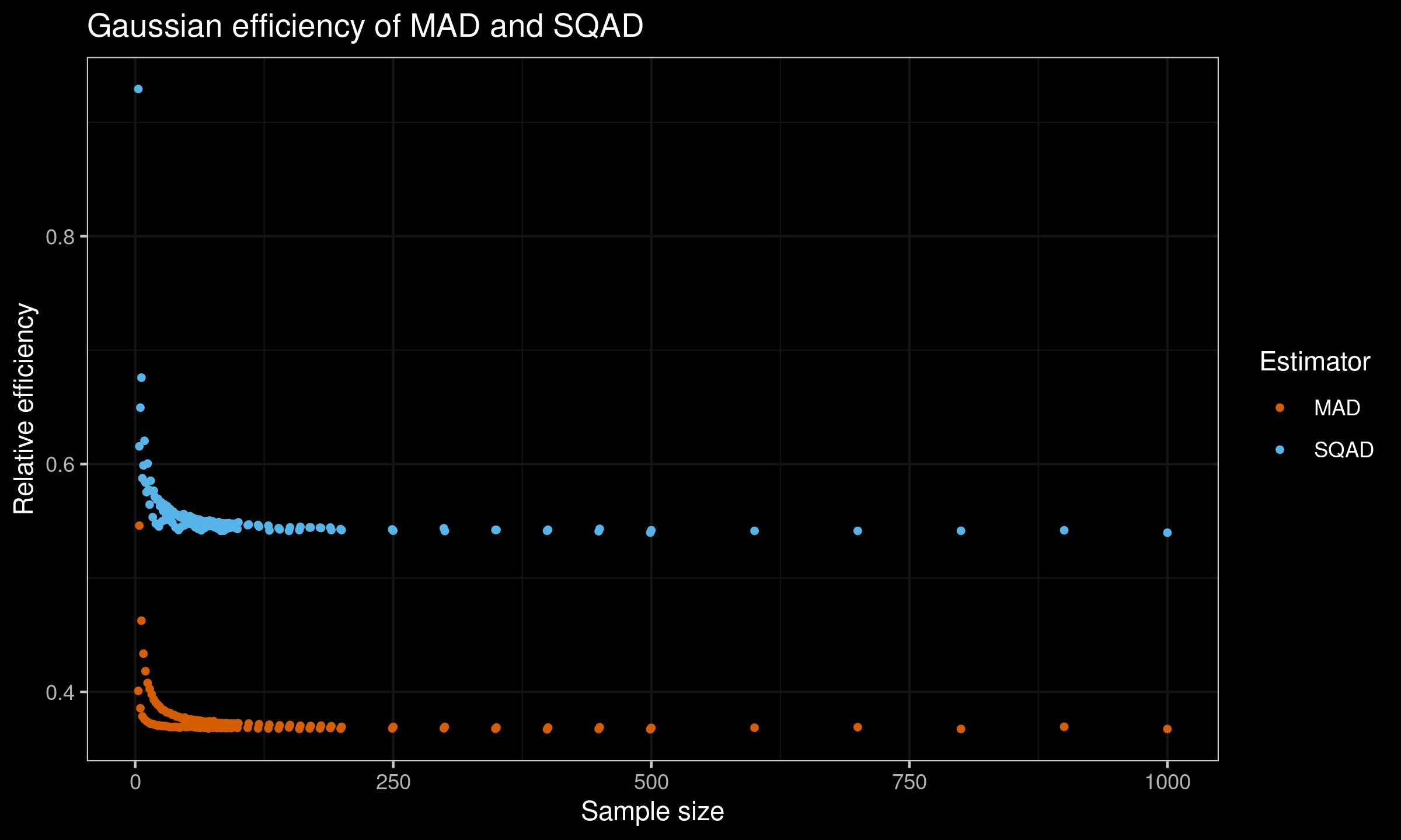
According to this simulation study, the Gaussian efficiency of $\SQAD$ is $\approx 54\%$.

Asymptotic efficiency of SQAD

We already know the equation for the Gaussian efficiency of $\QAD$:

$$ \lim_{n \to \infty} e(\QAD_n(X, p),\; \SD_n(X)) = \Bigg( \pi p(1-p) \exp\Big(2\big(\erfinv(p) \big)^2 \Big) \Bigg)^{-1}. $$

To adopt this equation for $\SQAD$, we should put $p = \Phi(1) - \Phi(-1)$.

Since $\Phi(1) = (1 + \erf(1/\sqrt{2})) / 2$, we can write

$$ \erf(1/\sqrt{2}) = 2\Phi(1) - 1 = \Phi(1) - \Phi(-1), $$

which is the same as

$$ 2\Big(\erfinv(\Phi(1) - \Phi(-1)) \Big)^2 = 1. $$

This gives us a simple expression for the Gaussian efficiency of $\SQAD_n(X)$:

$$ \lim_{n \to \infty} e(\SQAD_n(X),\; \SD_n(X)) = \Big( \pi e \cdot (\Phi(1)-\Phi(-1)) \cdot (1-\Phi(1)+\Phi(-1)) \Big)^{-1} \approx 0.540565. $$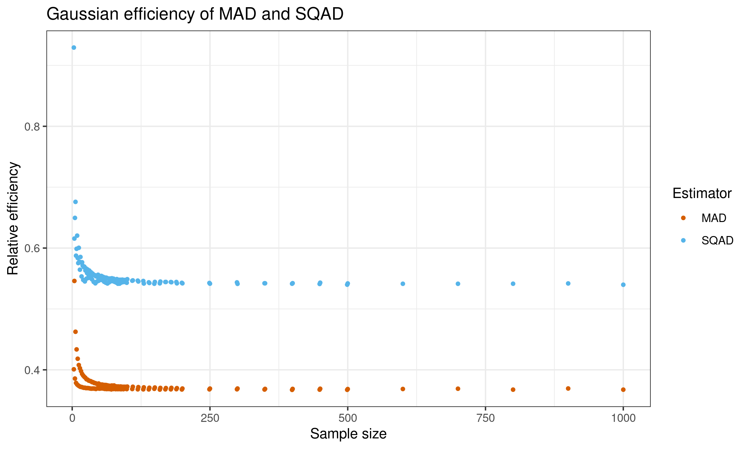

Summary

In this post, we discussed a new measure of statistical dispersion called the standard quantile absolute deviation ($\SQAD$) which is consistent with the standard deviation under normality. Its breakdown point is $\approx 31.73\%$. When such robustness is enough, $\SQAD$ can be a decent replacement for the median absolute deviation because it has higher statistical efficiency ($\approx 54\%$).

References

• [Hyndman1996]
  Hyndman, R. J. and Fan, Y. 1996. Sample quantiles in statistical packages, American Statistician 50, 361–365.
  https://doi.org/10.2307/2684934
• [Harrell1982]
  Harrell, F.E. and Davis, C.E., 1982. A new distribution-free quantile estimator. Biometrika, 69(3), pp.635-640.
  https://pdfs.semanticscholar.org/1a48/9bb74293753023c5bb6bff8e41e8fe68060f.pdf
• [Akinshin2022]
  Andrey Akinshin (2022) Trimmed Harrell-Davis quantile estimator based on the highest density interval of the given width, Communications in Statistics - Simulation and Computation.
  https://doi.org/10.1080/03610918.2022.2050396
• [Arnold2008]
  Arnold, Barry C., N. Balakrishnan, and H. N. Nagaraja. A First Course in Order Statistics. Classics in Applied Mathematics 54. Philadelphia, PA: SIAM, 2008.