Statistical approaches for performance analysis
Software performance is a complex discipline that requires knowledge in different areas from benchmarking to the internals of modern runtimes, operating systems, and hardware. Surprisingly, the most difficult challenges in performance analysis are not about programming, they are about mathematical statistics!
Many software developers can drill into performance problems and implement excellent optimizations, but they are not always know how to correctly verify these optimizations. This may not look like a problem in the case of a single performance investigation. However, the situation became worse when developers try to set up an infrastructure that should automatically find performance problems or prevent degradations from merging. In order to make such an infrastructure reliable and useful, it’s crucial to achieve an extremely low false-positive rate (otherwise, it’s not trustable) and be able to detect most of the degradations (otherwise, it’s not so useful). It’s not easy if you don’t know which statistical approaches should be used. If you try to google it, you may find thousands of papers about statistics, but only a small portion of them really works in practice.
In this post, I want to share some approaches that I use for performance analysis in everyday life. I have been analyzing performance distributions for the last seven years, and I have found a lot of approaches, metrics, and tricks which nice to have in your statistical toolbox. I would not say that all of them are must have to know, but they can definitely help you to improve the reliability of your statistical checks in different problems of performance analysis. Consider the below list as a letter to a younger version of myself with a brief list of topics that are good to learn.
Bad approaches
The classic statistics aggressively promotes a lot of approaches that don’t work well on performance distributions. I’m not sure that I know the best tools for performance analysis, but I’m sure that I know dozens of approaches that shouldn’t be used. Let me briefly highlight the most popular sources of trouble.
Don’t assume normal distributions
The first thing you should remember about performance distributions: they are not normal. Of course, some of them could remind the normal distribution, but you can’t assume normality in advance. Performance distributions can be asymmetric and heavy-tailed, can contain extremely high outliers, can be multimodal, can have a strange distribution shape.
Thus, it’s not a good idea to use any approaches that require normality. Instead, you should look for distribution-free methods that support non-parametric distributions.
References:
- Normality is a myth
- Testing for normality (1947) by R.C. Geary
- Introduction to Robust Estimation and Hypothesis Testing (4th edition) Rand R. Wilcox
Don’t use null hypothesis significance testing with p-values
The null hypothesis significance testing (NHST) is an awful technique that typically creates more problems than solves. I had been using it for many years, I had been trying a lot of different tests, and now I am completely disappointed in this.
To be honest, if you aware of all the possible pitfalls, it’s possible to conduct a good performance analysis with NHST. Note that most of the significance tests assume normality, so if you decide to use NHST, make sure that you use non-parametric tests (e.g., the Mann–Whitney U test or the Kolmogorov–Smirnov test).
However, there are other approaches that are much more reliable than NHST. For example, you can look at the Bayesian statistics and the Estimation statistics (also known as the new statistics).
If you use NHST, I highly recommend to read the following books and papers:
- What If There Were No Significance Tests? (1997) by Lisa L. Harlow, Stanley A. Mulaik, James H. Steiger
- Amrhein, Valentin, Fränzi Korner-Nievergelt, and Tobias Roth. “The earth is flat (p> 0.05): significance thresholds and the crisis of unreplicable research.” PeerJ 5 (2017): e3544.
https://peerj.com/articles/3544/ - Wasserstein, Ronald L., Allen L. Schirm, and Nicole A. Lazar. “Moving to a world beyond “p< 0.05”.” (2019): 1-19.
https://www.tandfonline.com/doi/full/10.1080/00031305.2019.1583913 - Matthews, Robert AJ. “Moving towards the post p< 0.05 era via the analysis of credibility.” The American Statistician 73, no. sup1 (2019): 202-212.
https://www.tandfonline.com/doi/full/10.1080/00031305.2018.1543136 - Andrade, Chittaranjan. “The P value and statistical significance: misunderstandings, explanations, challenges, and alternatives.” Indian Journal of Psychological Medicine 41, no. 3 (2019): 210-215. https://www.ncbi.nlm.nih.gov/pmc/articles/PMC6532382/
- Winder, W. C. “What you always wanted to know about testing but were afraid to ask.” American dairy review (1973).
https://www.researchgate.net/publication/241372934 - Grieve, Andrew P. “How to test hypotheses if you must.” Pharmaceutical statistics 14, no. 2 (2015): 139-150.
http://doi.wiley.com/10.1002/pst.1667 - Krawczyk, Michał. “The search for significance: a few peculiarities in the distribution of P values in experimental psychology literature.” PloS one 10, no. 6 (2015).
https://dx.plos.org/10.1371/journal.pone.0127872 - “Still Not Significant” by Matthew Hankins
https://mchankins.wordpress.com/2013/04/21/still-not-significant-2/
A few good books about alternative approaches:
- Understanding the New Statistics: Effect Sizes, Confidence Intervals, and Meta-Analysis (2011) by Geoff Cumming
- Doing Bayesian Data Analysis: A Tutorial Introduction with R (2010) by John K. Kruschke
- Introduction to Robust Estimation and Hypothesis Testing (2017, 4th edition) Rand R. Wilcox
Don’t use non-robust metrics and approaches
If your performance metrics can be spoiled by a single outlier value, these metrics are not robust. If you use robust statistics, a lot of nasty problems will be resolved automatically.
Basic descriptive analysis
Now it’s time to talk about good approaches for descriptive analysis of your distributions.
Central tendency: the median instead of the mean
The arithmetic mean is not robust metric. It can be spoiled by a single outlier, which makes it unreliable. Instead of the mean, it’s much better to use the median, which is much more robust.
Quantile analysis
In the case of non-parametric distributions, you can’t describe your distribution by a limited number of parameters (that’s why they are called non-parametric). It’s recommended to use all the quantile values instead of a single median value.
The Harrell-Davis quantile estimator
The default quantile estimators that can be found in many programming languages are not so good. They are typically based on linear interpolation of two subsequent elements, and they don’t provide a good estimation of the actual quantile values.
To improve the situation, it’s recommended to use the Harrell-Davis quantile estimator. It’s more robust, and it provides better quantile estimations.
References:
- Harrell, F.E. and Davis, C.E., 1982. A new distribution-free quantile estimator.
Biometrika, 69(3), pp.635-640.
https://pdfs.semanticscholar.org/1a48/9bb74293753023c5bb6bff8e41e8fe68060f.pdf
The Maritz-Jarrett method for quantile confidence interval estimations
It’s also important to know how to estimate confidence intervals around the given quantiles. Based on my experience, one of the best solutions for this is the Maritz-Jarrett method.
- Maritz, J. S., and R. G. Jarrett. 1978.
“A Note on Estimating the Variance of the Sample Median.”
Journal of the American Statistical Association 73 (361): 194–196.
https://doi.org/10.1080/01621459.1978.10480027 - Introduction to Robust Estimation and Hypothesis Testing (2017, 4th edition) Rand R. Wilcox
Dispersion: the median absolute deviation instead of the standard deviation
Typically, people use the standard deviation as a measure of the statistical dispersion. It works great for normal distribution, but it may be very misleading in the case of non-parametric distribution. It’s recommended to use alternative measures of dispersion such as the median absolute deviation. The efficiency of this metric can be significantly improved with the help of the Harrell-Davis quantile estimator.
Quantile absolute deviation
In classic statistics, the median absolute deviation is calculated around the median value. However, we can calculate the median absolute deviation around any quantile. We can also calculate the quantile absolute deviation which provides a more robust set of dispersion values for the given quantile.
Extreme value theory for higher quantile estimations
The above methods allow getting an accurate estimation and a confidence interval around the median value. However, if you apply these techniques to higher quantiles (e.g., 95th, 99th, or 99.9th percentiles), you may get inaccurate values that can’t be trusted. To get better estimations, you can approximate tails of your distributions using the extreme value theory.
References:
- Statistical Analysis of Extreme Values: With Applications to Insurance, Finance, Hydrology and Other Fields (2007) by Rolf-Dieter Reiß, Michael Thomas
Quantile-respectful density plots
It’s also important to know how to visualize the density plot for your distributions. Typically, people use histograms and kernel density estimations (KDE). Unfortunately, these visualizations require tricky parameter tuning. If you plot a histogram or a KDE using the default settings, you may easily get a misleading chart. To prevent such problems, I prefer using the quantile-respectful density plots based on the Harrell-Davis quantile estimators.
References:
- Misleading histograms
- The importance of kernel density estimation bandwidth
- Quantile-respectful density estimation based on the Harrell-Davis quantile estimator
Outlier detection
Many statistical techniques don’t work well when you have outliers (extreme values). Thus, it’s good to know how to detect such values. Unfortunately, most popular approaches like Tukey’s fences may produce strange results on multimodal distributions. If you are looking for a simple and fast outlier checker, you can use DoubleMAD outlier detector based on the Harrell-Davis quantile estimator. You can also achieve better results in outlier detection using different techniques from the cluster analysis.
Note that outliers are not always extremely low or high values. In the case of multimodal distributions, you may also have intermodal outliers.
Highest density intervals
It’s also important to know how to report ranges that cover the major part of the distribution. If you just report the minimum and the maximum, you may get a misleading range because of the outliers. Of course, you can just remove outliers and report the min/max for the rest of the collected values, but this approach is not robust. One of the alternative approaches is to use the highest density intervals (HDI). It’s a variation of the credible intervals from the Bayesian statistics.
References:
- Doing Bayesian Data Analysis: A Tutorial Introduction with R (2010) by John K. Kruschke
Multimodality detection
Multimodality is one of the biggest challenges in performance analysis. If your distribution is multimodal, it makes most of your metrics such as the median and the median absolute deviation. To prevent such situations, you should check the distribution modality first. I didn’t find any workable approaches on the internet, so I came up with my own: Lowland multimodality detection.
When you process hundreds of different distribution each day, it may be inconvenient to look at the density plots for each distribution. In most cases, I prefer to work with command-line or plain text reports. So, I also came up with a plain text notation for multimodality distributions that significantly simplifies the analysis routine.
Comparing distributions
Now we know about methods that can be used to describe a single distribution. Let’s say that we have two distributions, and we want to compare them. How should we do it?
Shift and ratio functions
One of my favorite approaches is to use the shift and ration functions. The idea is simple: we should just calculate all the quantiles for each distribution and compare them! The shift functions show the absolute difference between quantiles. The ratio functions show the relative difference between quantiles.
Effect sizes
It’s not always easy to work with absolute/relative quantile differences because it’s hard to specify thresholds. 1 millisecond may be a huge difference for a nano-benchmark, and it may be insignificant for a benchmark that takes minutes. 10% may be a huge difference for a benchmark with a small dispersion (e.g., around 1% of the quantile value), and it may be insignificant for a benchmark with a huge dispersion (e.g., around 300% of the quantile value).
The effect size resolves this problem. In most cases, it’s just the absolute difference normalized by the dispersion. The effect sizes report the difference using abstract units that have the same meaning for all kinds of distributions.
Quantile-specific effect sizes
Unfortunately, most of the classic effect size equations assume normal distributions and estimate the difference between the distribution mean values. So, I came up with a generalization of Cohen’s d (which is one of the most popular measures of the effect size) that supports non-parametric distributions and estimates the difference between given quantiles.
References:
Other useful approaches
In addition, I want to say a few words about other approaches that can also be extremely useful in performance analysis.
Sequential analysis
Let’s say you want to execute several iterations of a benchmark. How many iterations should you run? If the number of iterations is too low, you may get unreliable statistical metrics. If the number of iterations is too big, you will wait for the benchmark results too long without visible benefits in terms of accuracy. Unfortunately, you can’t predict the perfect number of iterations in advance because you don’t know the exact distribution form for your benchmark.
This problem can be solved using the sequential analysis and optimal stopping. The idea is simple. After each iteration, we should reevaluate statistical metrics and make a decision: do we need one more iteration or not.
Weighted samples
Now imagine that you collect some performance measurements every day on your CI server. Each day you get a small sample of values that is not enough to get the accurate daily quantile estimations. However, the full time-series over the last several weeks has a decent size. You suspect that past measurements should be similar to today measurements, but you are not 100% sure about it. You feel a temptation to extend the up-to-date sample by the previously collected values, but it may spoil the estimation (e.g., in the case of recent change points or positive/negative trends).
One of the possible approaches in this situation is to use weighted samples. This assumes that we add past measurements to the “today sample,” but these values should have a smaller weight. The older measurement we take, the smaller weight it gets. If you have consistent values across the last several days, this approach works like a charm. If you have any recent changes, you can detect such situations by huge confidence intervals due to the sample inconsistency.
To determine the exact weights for each measurement, I prefer using the exponential decay.
It’s also worth to note that the Harrell-Davis quantile estimator and the Maritz-Jarrett method can be generalized to the weighed case (see Weighted quantile estimators and Quantile confidence intervals for weighted samples ).
Change point detection
Let’s say you want to analyze the history of your performance values and find moments when the form of the underlying distribution was changed. For this problem, you need a change point detection (CPD) algorithm.
There are a lot of different CPD algorithms (e.g., you can find a good overview in Selective review of offline change point detection methods
By Charles Truong, Laurent Oudre, Nicolas Vayatis
·
2020truong2020:
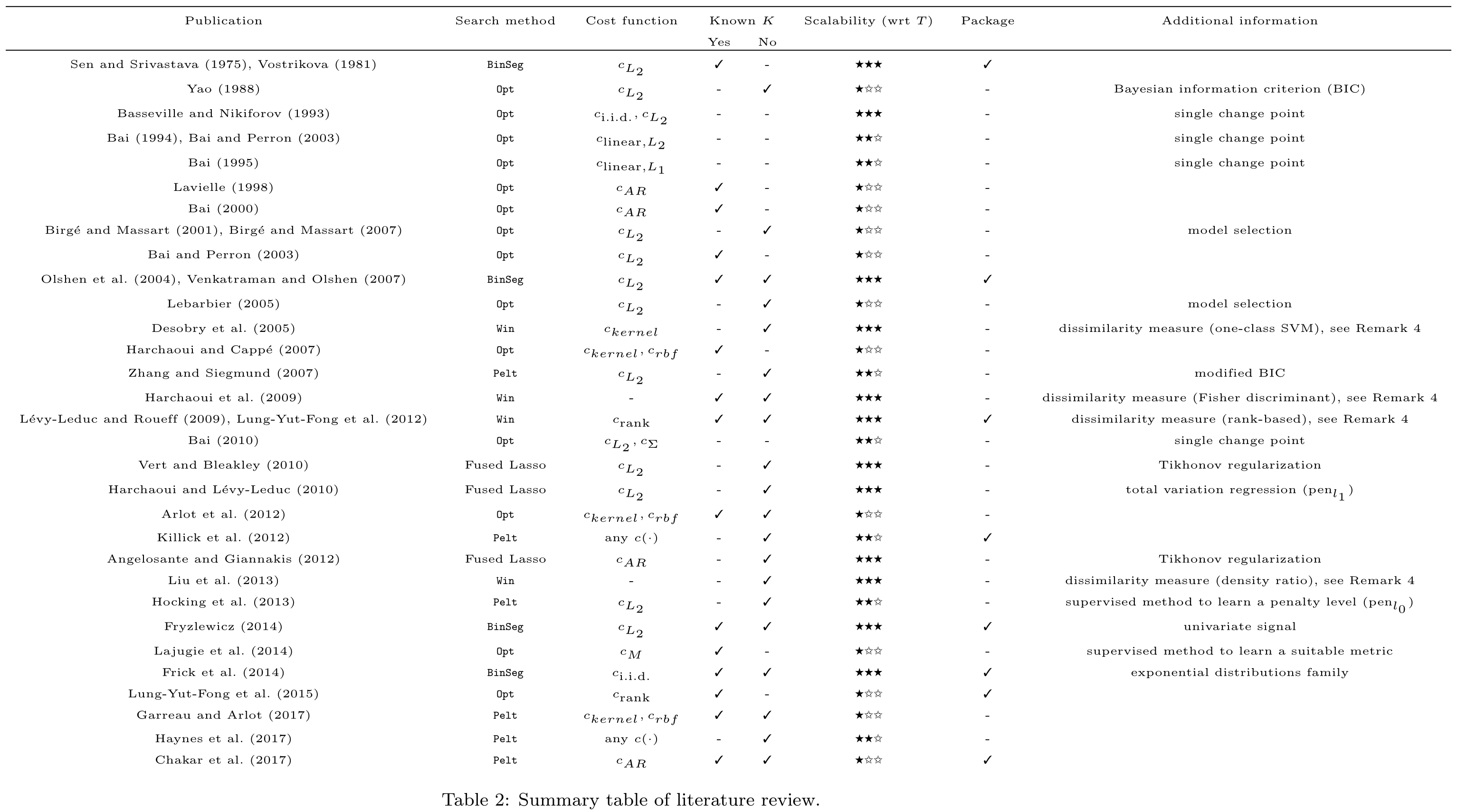
From all the algorithms I tried, I found the only one that satisfied me in terms of speed and accuracy: ED-PELT (an implementation can be found here). Unfortunately, it didn’t work well on long time-series with a high number of change points. So, I came up with my own algorithm called RqqPelt. I haven’t written a post/paper about it yet, but you can try it yourself with the help of perfolizer.
References:
- Truong, Charles, Laurent Oudre, and Nicolas Vayatis. “Selective review of offline change point detection methods.” Signal Processing 167 (2020): 107299.
https://arxiv.org/pdf/1801.00718.pdf - Haynes, Kaylea, Paul Fearnhead, and Idris A. Eckley. “A computationally efficient nonparametric approach for changepoint detection.” Statistics and Computing 27, no. 5 (2017): 1293-1305.
https://link.springer.com/article/10.1007/s11222-016-9687-5
Streaming quantile estimators
Imagine that you are implementing performance telemetry in your application. There is an operation that is executed millions of times, and you want to get its “average” duration. It’s not a good idea to use the arithmetic mean because the obtained value can be easily spoiled by outliers. It’s much better to use the median which is one of the most robust ways to describe the average.
The straightforward median estimation approach requires storing all the values. In our case, it’s a bad idea to keep all the values because it will significantly increase the memory footprint. Such telemetry is harmful because it may become a new bottleneck instead of monitoring the actual performance.
Another way to get the median value is to use a sequential quantile estimator (also known as an online quantile estimator or a streaming quantile estimator).
There are a lot of good sequential quantile estimators that work well. One of my favorites is the P² quantile estimator because it has low overhead and it’s very simple.
Conclusion
In this post, I covered some of the statistical approaches that I use for performance analysis. This list is based on real-life experience. It worth to say that if you conduct a performance investigation one time per month, you probably don’t actually need all these metrics and approaches. However, if you want to set up a reliable infrastructure for performance monitoring that processes thousands of distribution each day, robust non-parametric approaches are required. Without them, you can’t achieve a decent level of reliability.
Several month ago, I have decided to implement the most useful algorithms and assemble them in a single place. So, if you are looking for reference implementations of the above algorithms, you can check out perfolizer. Note that most of the approaches are available only in the nightly versions, but I’m going to release a new stable version soon. Keep tuned!