Standard trimmed Harrell-Davis median estimator

In one of the previous posts, I suggested a new measure of dispersion called the standard quantile absolute deviation around the median ($\operatorname{SQAD}$) which can be used as an alternative to the median absolute deviation ($\operatorname{MAD}$) as a consistent estimator for the standard deviation under normality. The Gaussian efficiency of $\operatorname{SQAD}$ is $54\%$ (comparing to $37\%$ for MAD), and its breakdown point is $32\%$ (comparing to $50\%$ for MAD). $\operatorname{SQAD}$ is a symmetric dispersion measure around the median: the interval $[\operatorname{Median} - \operatorname{SQAD}; \operatorname{Median} + \operatorname{SQAD}]$ covers $68\%$ of the distribution. In the case of the normal distribution, this corresponds to the interval $[\mu - \sigma; \mu + \sigma]$.

If we use $\operatorname{SQAD}$, we accept the breakdown point of $32\%$. This makes the sample median a non-optimal choice for the median estimator. Indeed, the sample median has high robustness (the breakdown point is $50\%$), but relatively poor Gaussian efficiency. If we use $\operatorname{SQAD}$, it doesn’t make sense to require a breakdown point of more than $32\%$. Therefore, we could trade the median robustness for efficiency and come up with a complementary measure of the median for $\operatorname{SQAD}$.

In this post, we introduce the standard trimmed Harrell-Davis median estimator which shares the breakdown point with $\operatorname{SQAD}$ and provides better finite-sample efficiency comparing to the sample median.

Trimmed Harrell-Davis quantile estimator

The concept of this estimator is fully covered in my recent paper [Akinshin2022]. Here I just briefly recall the basic idea.

Let $x$ be a sample with $n$ elements: $x = \{ x_1, x_2, \ldots, x_n \}$. We assume that all sample elements are sorted ($x_1 \leq x_2 \leq \ldots \leq x_n$) so that we could treat the $i^\textrm{th}$ element $x_i$ as the $i^\textrm{th}$ order statistic $x_{(i)}$. Based on the given sample, we want to build an estimation of the $p^\textrm{th}$ quantile $Q(p)$.

The classic Harrell-Davis quantile estimator (see A new distribution-free quantile estimator
By Frank E Harrell, C E Davis · 1982harrell1982) suggests the following approach:

$$ Q_{\operatorname{HD}}(p) = \sum_{i=1}^{n} W_{\operatorname{HD},i} \cdot x_i,\quad W_{\operatorname{HD},i} = I_{i/n}(\alpha, \beta) - I_{(i-1)/n}(\alpha, \beta), $$

where $I_x(\alpha, \beta)$ is the regularized incomplete beta function, $\alpha = (n+1)p$, $\;\beta = (n+1)(1-p)$.

When we switch to the trimmed modification of this estimator, we perform summation only within the highest density interval $[L;R]$ of $\operatorname{Beta}(\alpha, \beta)$ of size $D$ (as a rule of thumb, we can use $D = 1 / \sqrt{n}$):

$$ Q_{\operatorname{THD},D}(p) = \sum_{i=1}^{n} W_{\operatorname{THD},D,i} \cdot x_i, \quad W_{\operatorname{THD},D,i} = F_{\operatorname{THD},D}(i / n) - F_{\operatorname{THD},D}((i - 1) / n), $$$$ F_{\operatorname{THD},D}(x) = \begin{cases} 0 & \textrm{for }\, x < L,\\ \big( I_x(\alpha, \beta) - I_L(\alpha, \beta) \big) / \big( I_R(\alpha, \beta) \big) - I_L(\alpha, \beta) \big) \big) & \textrm{for }\, L \leq x \leq R,\\ 1 & \textrm{for }\, R < x. \end{cases} $$

Thus, we use only sample elements with the highest weight coefficients ($W_{\operatorname{THD},D,i}$) and ignore sample elements with small weight coefficients. It allows us to get a high statistical efficiency (which is close to the efficiency of the classic Harrell-Davis quantile estimator) and a good robustness level (in most cases, outliers have zero impact on the final result).

Standard trimmed Harrell-Davis median estimator

The highest density interval size $D$ defines the portion of the sample that is actually used to estimate quantiles using $Q_{\operatorname{THD},D}$. Therefore, the asymptotic breakdown point of $Q_{\operatorname{THD},D}$ is $1-D$. In order to make $Q_{\operatorname{THD},D}$ consistent with $\operatorname{SQAD}$ in terms of robustness, we should use $D=\Phi(1)-\Phi(-1) \approx 0.6827$. We call such an estimator the standard trimmed Harrell-Davis median estimator and denote by $Q_{\operatorname{STHD}}$.

In the scope of this research, we are interested only in the median estimator $Q_{\operatorname{STHD}}(0.5)$. For the median estimator, the beta function $\operatorname{Beta}(\alpha, \beta)$ becomes symmetric around $0.5$ since $\alpha = \beta = (n + 1) / 2$; the interval $[L;R]$ becomes $[\Phi(-1); \Phi(1)]$.

$$ Q_{\operatorname{STHD}}(0.5) = \sum_{i=1}^{n} W_{\operatorname{STHD},i} \cdot x_i, \quad W_{\operatorname{STHD},i} = F_{\operatorname{STHD}}(i / n) - F_{\operatorname{STHD}}((i - 1) / n), $$$$ F_{\operatorname{STHD}}(x) = \begin{cases} 0 & \textrm{for }\, x < \Phi(-1),\\ \dfrac{ I_x(\frac{n+1}{2}, \frac{n+1}{2}) - I_L(\frac{n+1}{2}, \frac{n+1}{2}) }{I_R(\frac{n+1}{2}, \frac{n+1}{2}) - I_L(\frac{n+1}{2}, \frac{n+1}{2})} & \textrm{for }\, \Phi(-1) \leq x \leq \Phi(1),\\ 1 & \textrm{for }\, \Phi(1) < x. \end{cases} $$

Finite-sample efficiency of standard trimmed Harrell-Davis median estimator

In order to evaluate the actual finite-sample efficiency of $Q_{\operatorname{STHD}}(0.5)$, we perform a simple Monte-Carlo simulation. We enumerate various sample sizes; for each sample size we generate multiple random samples from the standard normal distribution; estimate the mean, the sample median, and $Q_{\operatorname{STHD}}(0.5)$; evaluate the relative efficiency of the sample median and $Q_{\operatorname{STHD}}(0.5)$ against the mean as the ratio of the corresponding variance values.

Here are the results for $n \leq 100$:

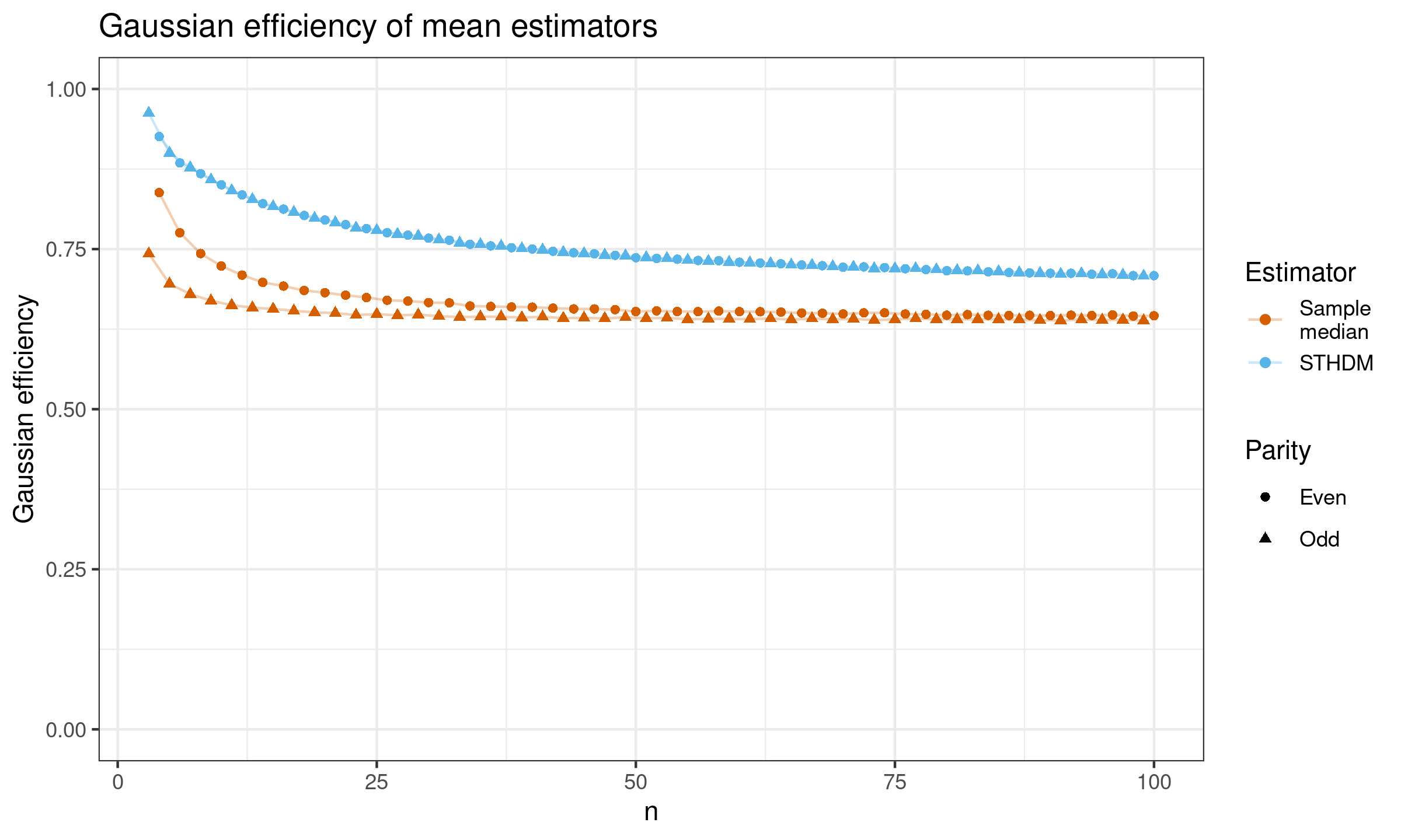
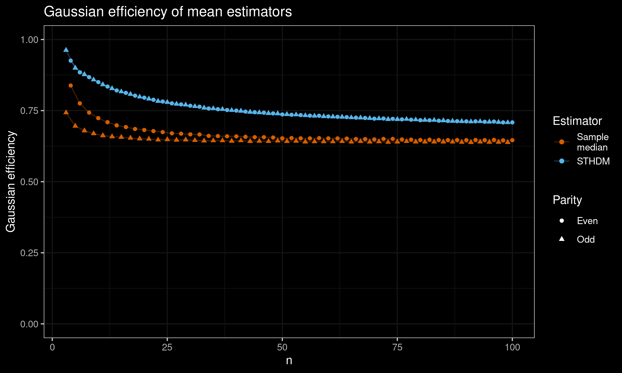
As we can see, for small samples, $Q_{\operatorname{STHD}}(0.5)$ is noticeably more efficient than the sample median.

And here are the results for $n \leq 100\,000$:

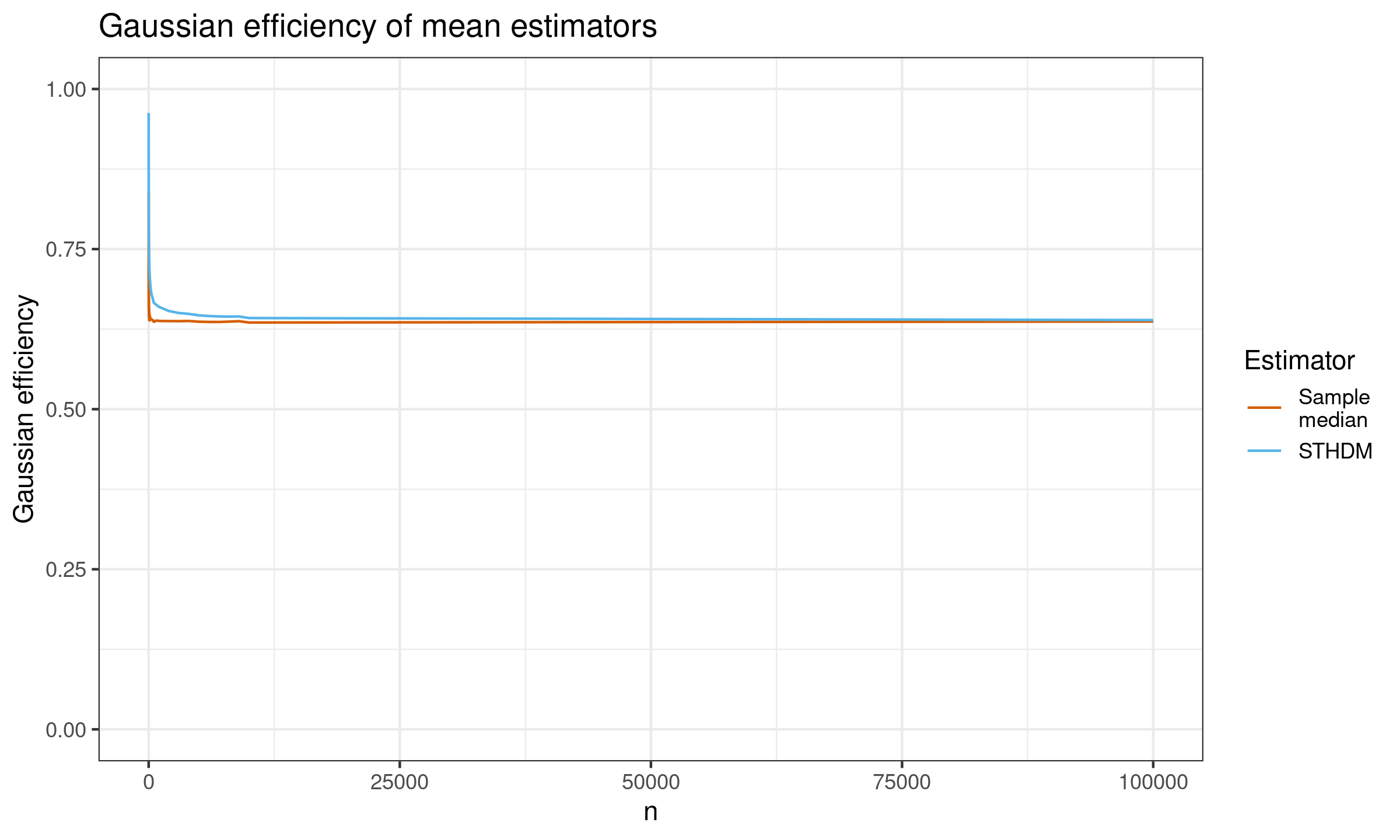
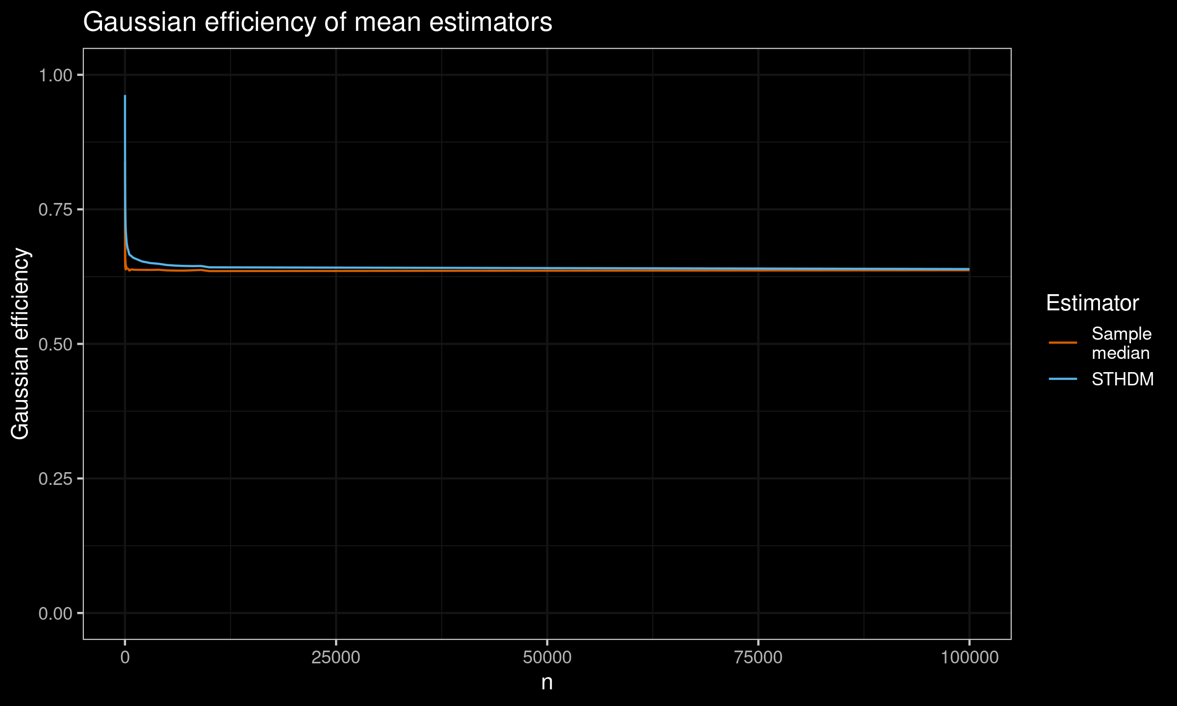
As we can see, asymptotically both estimators converge to the same value which is $2 / \pi \approx 63.66%$. It makes sense: the Harrell-Davis median estimator is asymptotically consistent with the traditional sample median (see Asymptotic equivalence of the Harrell-Davis median estimator and the sample median
By Carl N Yoshizawa, Pranab K Sen, C Edward Davis · 1985yoshizawa1985). Since $Q_{\operatorname{STHD}}(0.5)$ is “between” these two estimators, it is expected that all of them converge to the same value.

References

• [Akinshin2022]
  Andrey Akinshin (2022) Trimmed Harrell-Davis quantile estimator based on the highest density interval of the given width, Communications in Statistics - Simulation and Computation,
  DOI: 10.1080/03610918.2022.2050396
• [Yoshizawa1985]
  Carl N Yoshizawa, Pranab K Sen, and C Edward Davis. “Asymptotic equivalence of the Harrell- Davis median estimator and the sample median”. In: Communications in Statistics-Theory and Methods 14.9 (1985), pp. 2129–2136.
  https://doi.org/10.1080/03610928508829034
• [Harrell1982]
  Harrell, F.E. and Davis, C.E., 1982. A new distribution-free quantile estimator. Biometrika, 69(3), pp.635-640.
  https://doi.org/10.2307/2335999