Avoiding over-trimming with the trimmed Harrell-Davis quantile estimator

Previously, I already discussed the trimmed modification of the Harrell-Davis quantile estimator several times. I performed several numerical simulations that compare the statistical efficiency of this estimator with the efficiency of the classic Harrell-Davis quantile estimator (HDQE) and its winsorized modification; I showed how we can improve the efficiency using custom trimming strategies and how to choose a good trimming threshold value.

In the heavy-tailed cases, the trimmed HDQE provides better estimations than the classic HDQE because of its higher breakdown point. However, in the light-tailed cases, we could get efficiency that is worse than the baseline Hyndman-Fan Type 7 (HF7) quantile estimator. In many cases, such an effect arises because of the over-trimming effect. If the trimming percentage is too high or if the evaluated quantile is too far from the median, the trimming strategy based on the highest-density interval may lead to an estimation that is based on single order statistics. In this case, we get an efficiency level similar to the Hyndman-Fan Type 1-3 quantile estimators (which are also based on single order statistics). In the light-tailed case, such a result is less preferable than Hyndman-Fan Type 4-9 quantile estimators (which are based on two subsequent order statistics).

In order to improve the situation, we could introduce the lower bound for the number of order statistics that contribute to the final quantile estimations. In this post, I look at some numerical simulations that compare trimmed HDQEs with different lower bounds.

Simulation design

The basic settings for the simulation are the same ones that were used in the previous post. However, now we are going to compare the following quantile estimators:

• HD: the classic Harrell-Davis quantile estimator that is based on a weighted sum of all order statistics
• THD|0.5|Min1: the trimmed modification of the Harrell-Davis quantile estimator that is based on 50% highest density interval with lower bound = 1 (works the same way as trimmed HDQEs from previous posts)
• THD|0.5|Min2: the trimmed modification of the Harrell-Davis quantile estimator that is based on 50% highest density interval with lower bound = 2 (always uses at least 2 order statistics)
• THD|0.5|Min3: the trimmed modification of the Harrell-Davis quantile estimator that is based on 50% highest density interval with lower bound = 3 (always uses at least 3 order statistics)

Let’s look at the results!

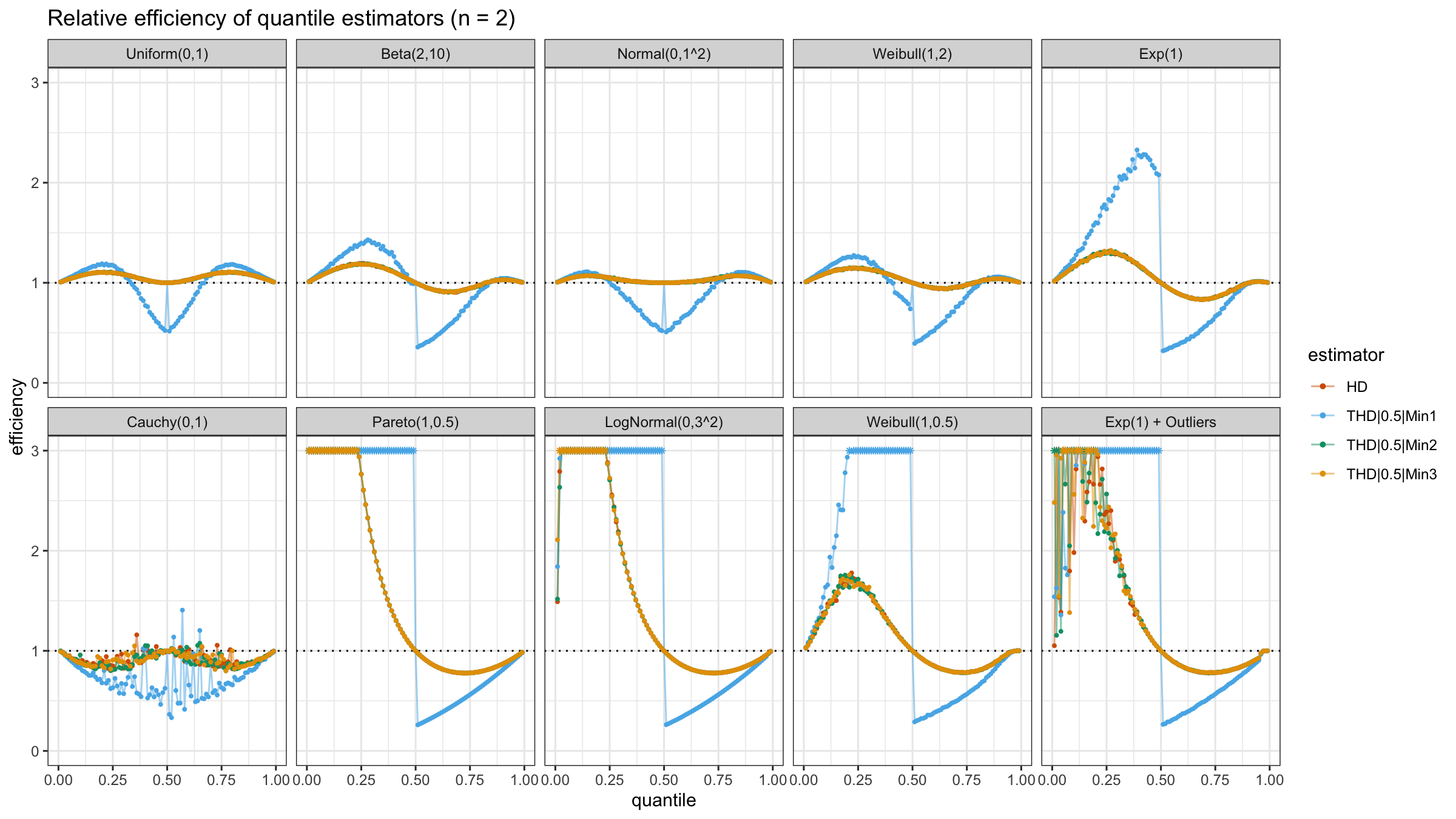
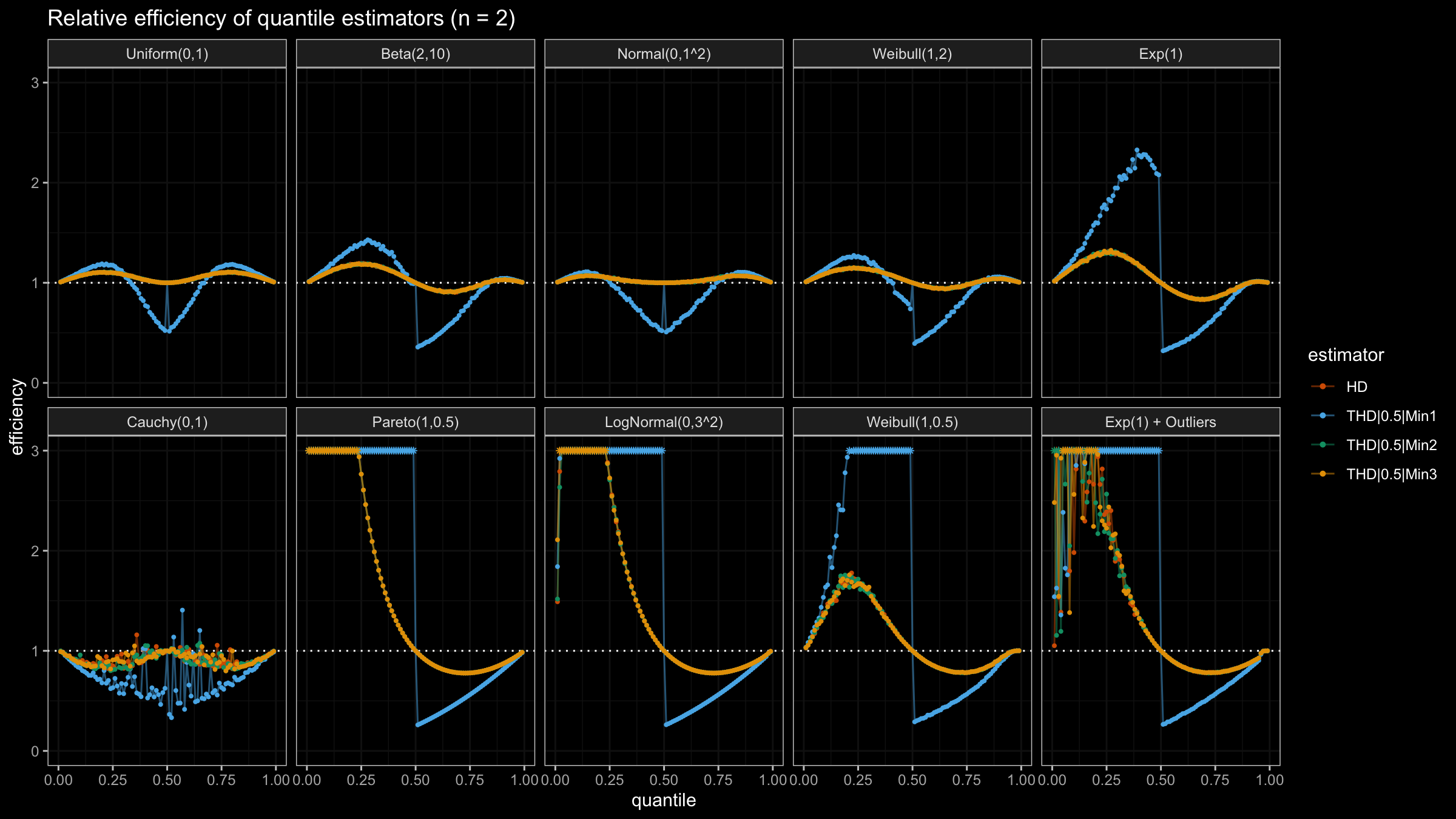
N=2

With N=2, HD, THD|0.5|Min2, and THD|0.5|Min3 work the same way: all of them always use both sample elements, unlike THD|0.5|Min1 that can use only a single element. Obviously, THD|0.5|Min1 “wins” when we evaluate lower quantiles of heavy-tailed distributions because of its higher robustness level. Unfortunately, it provides poor median estimations in the light-tailed cases.

N=3

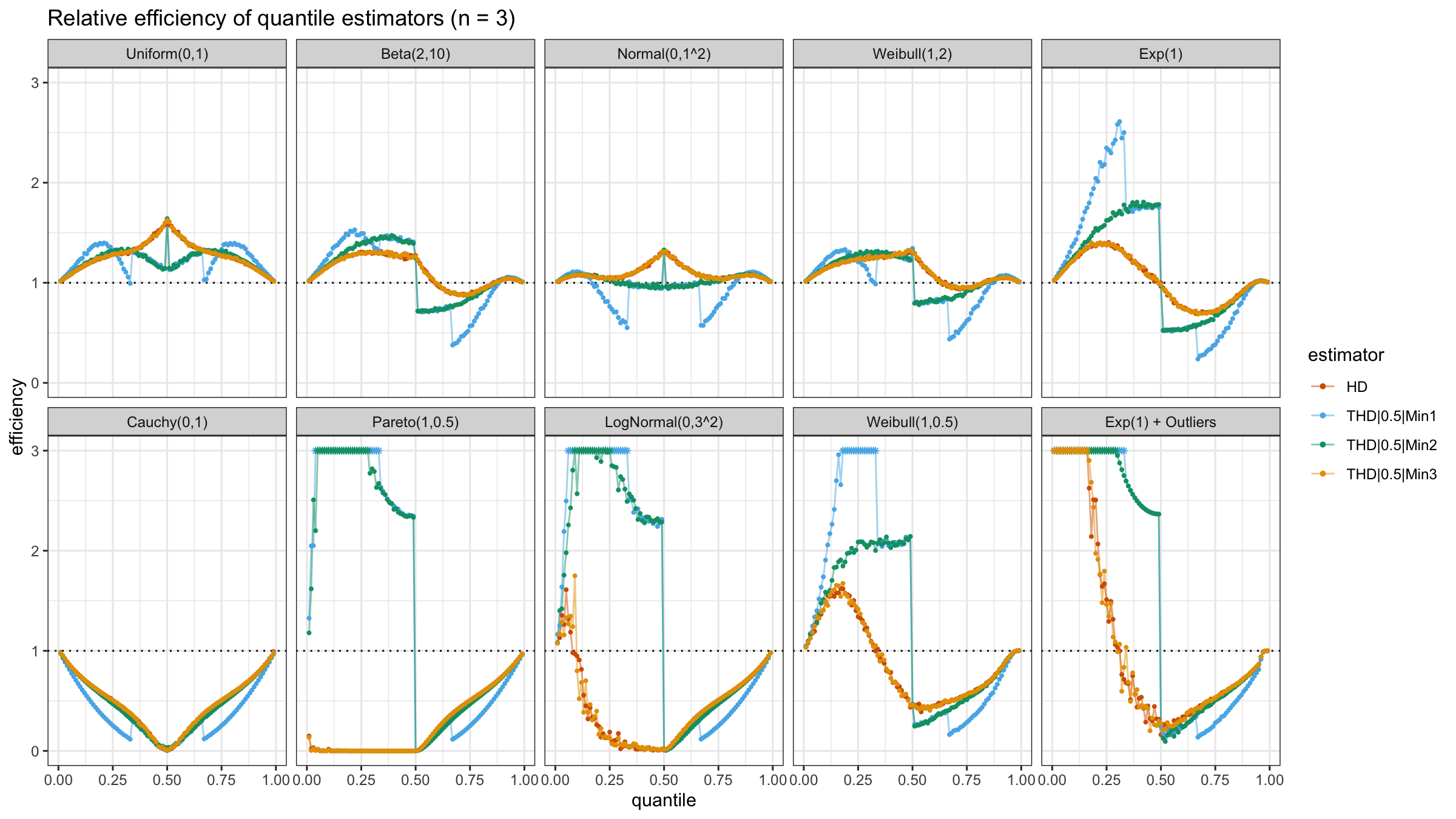
With N=3, HD and THD|0.5|Min3 still work the same way (both of them always use all sample elements). THD|0.5|Min2 and THD|0.5|Min1 works pretty good on lower quantiles of heavy-tailed distributions and not-so-good with light-tailed distributions. However, THD|0.5|Min2 shows better results than THD|0.5|Min1 because it always uses at least two order statistics.

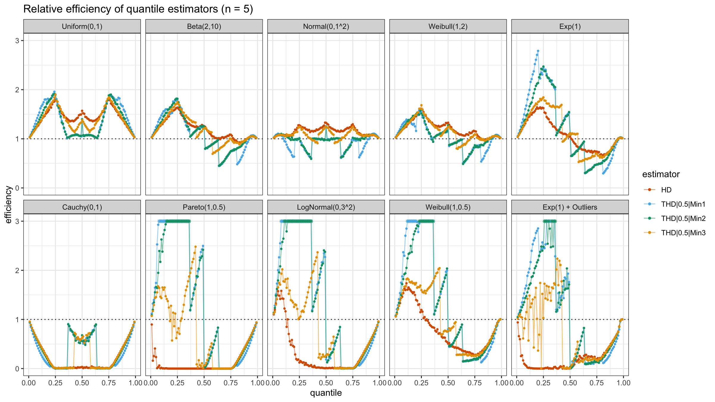
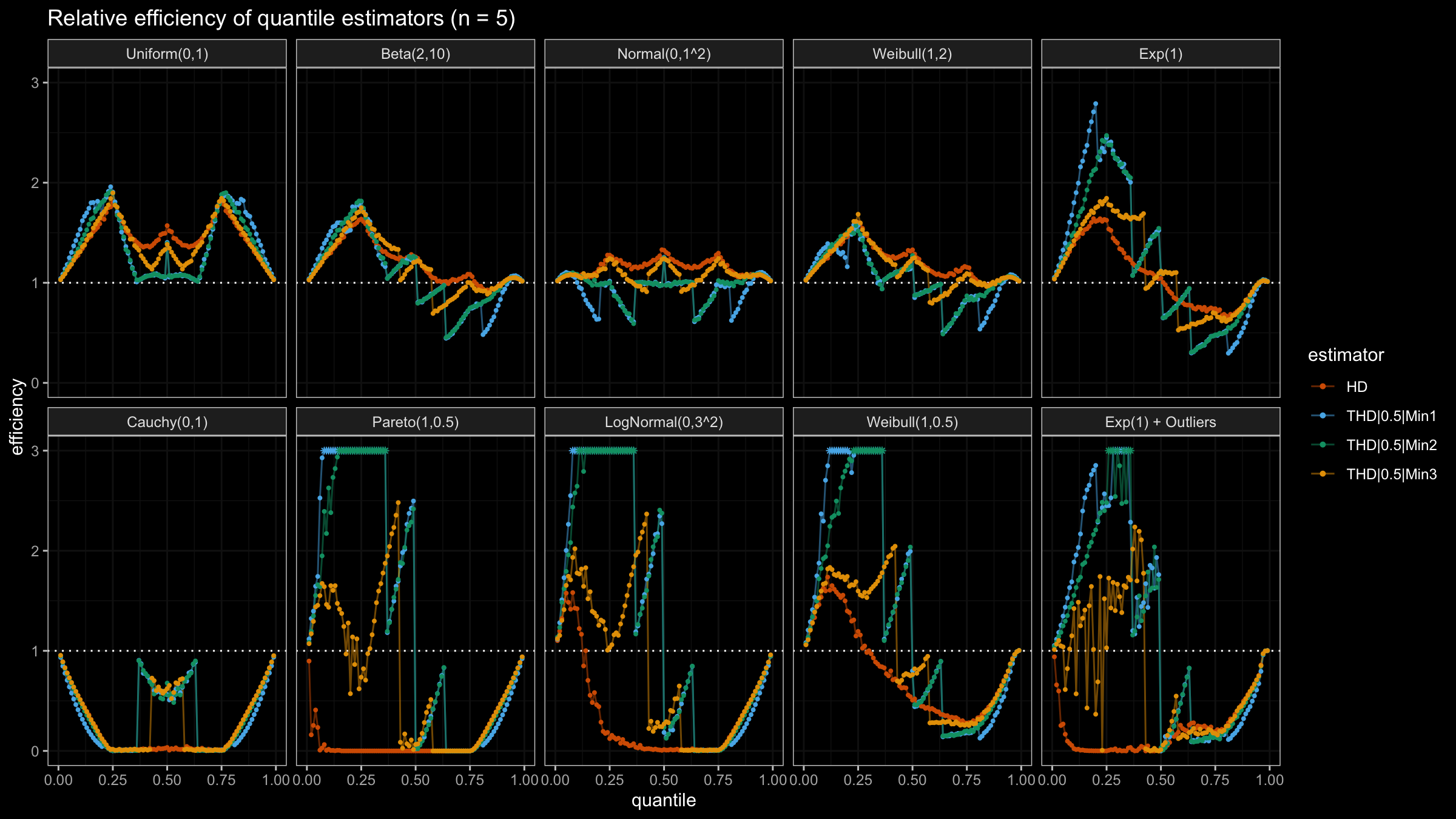
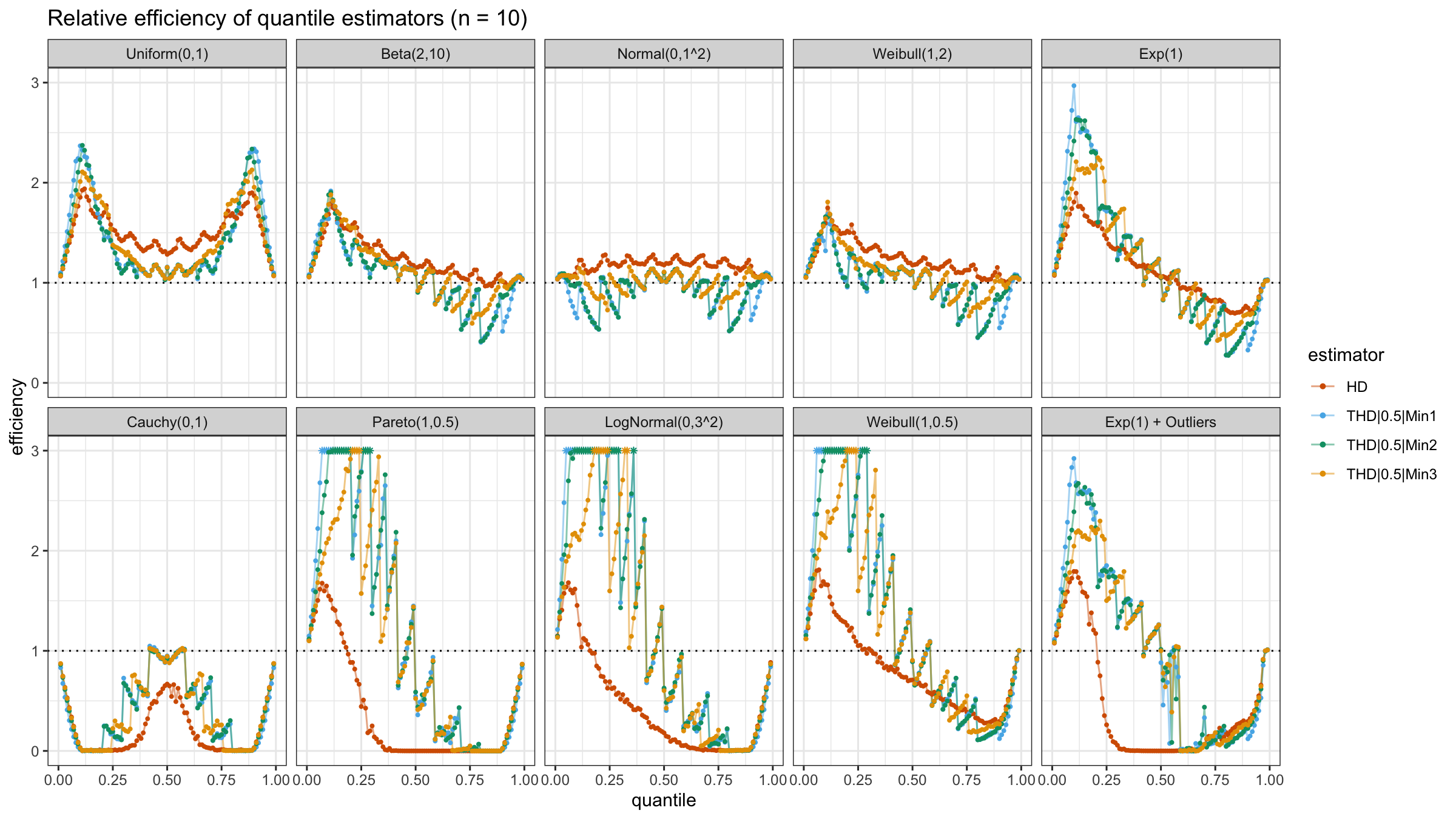
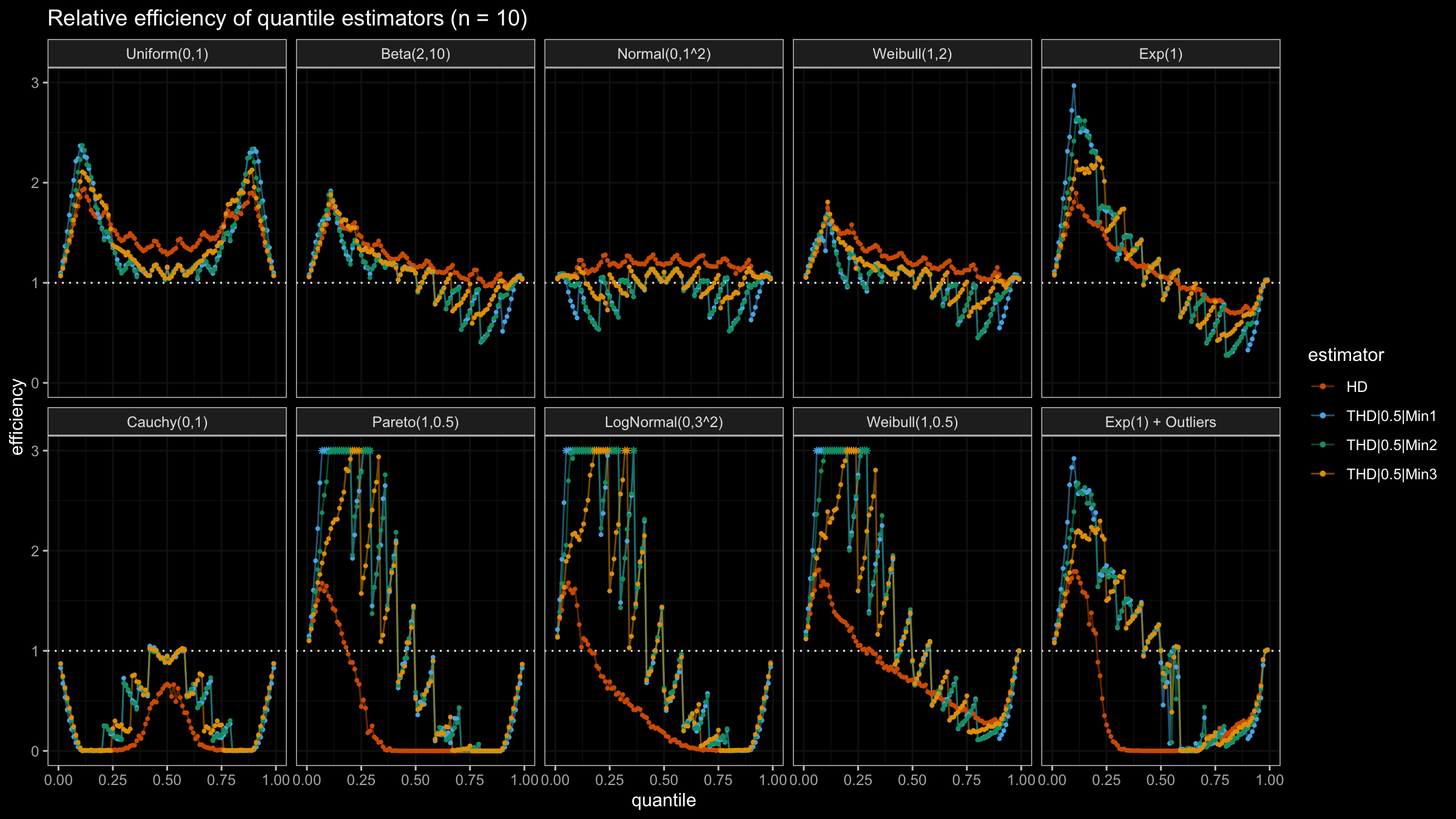
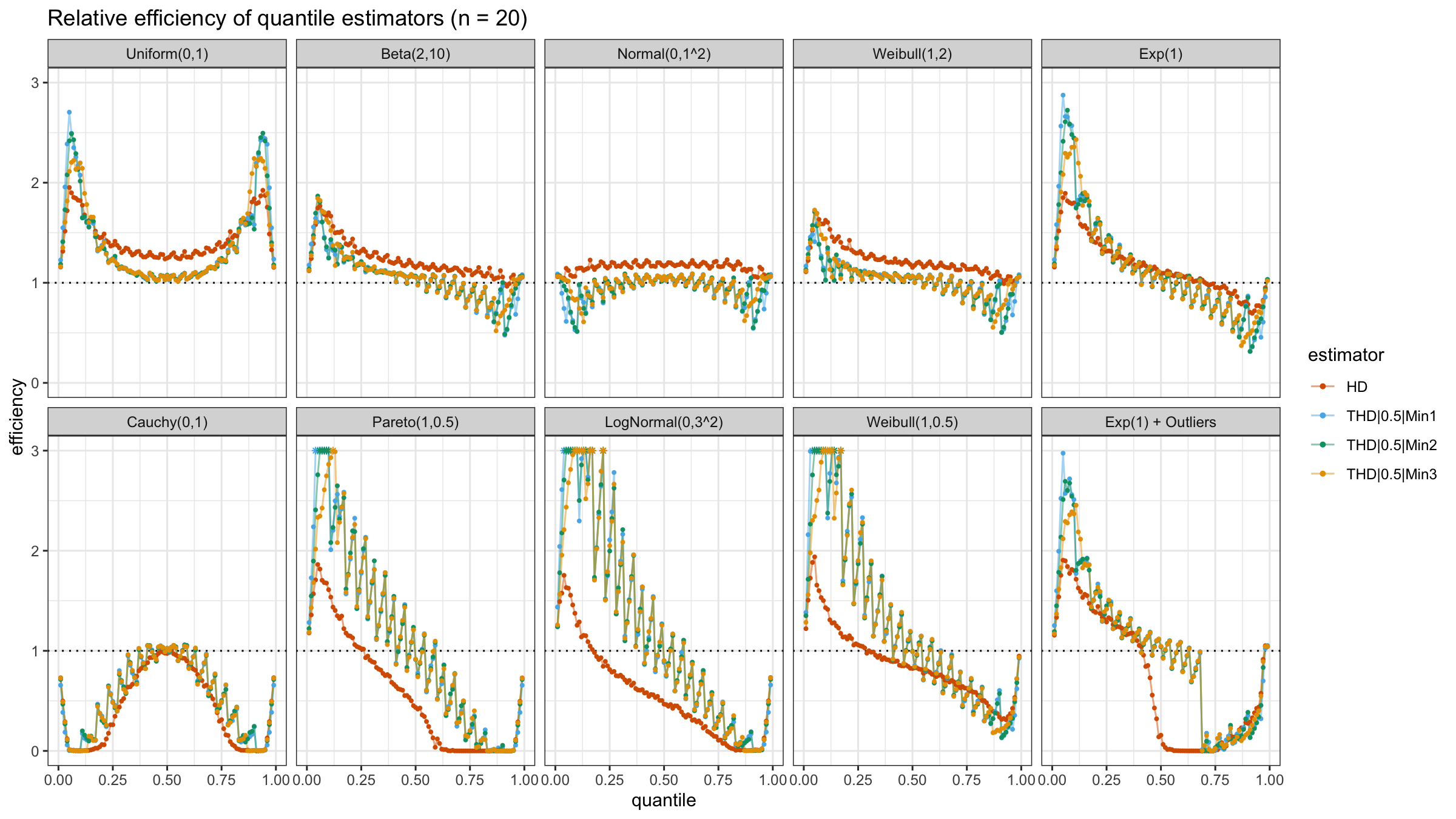
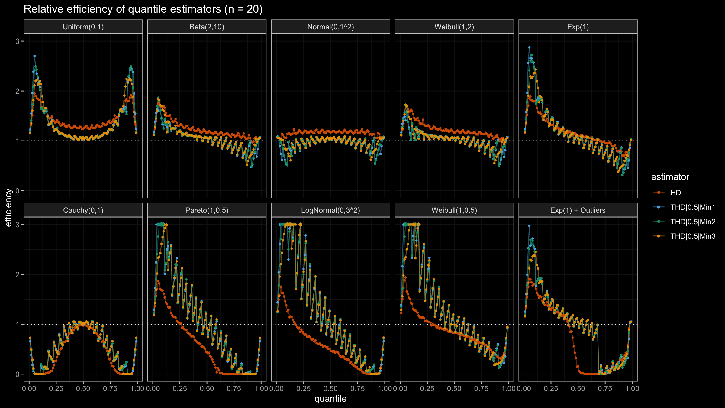
N=4, N=5, N=10, N=20

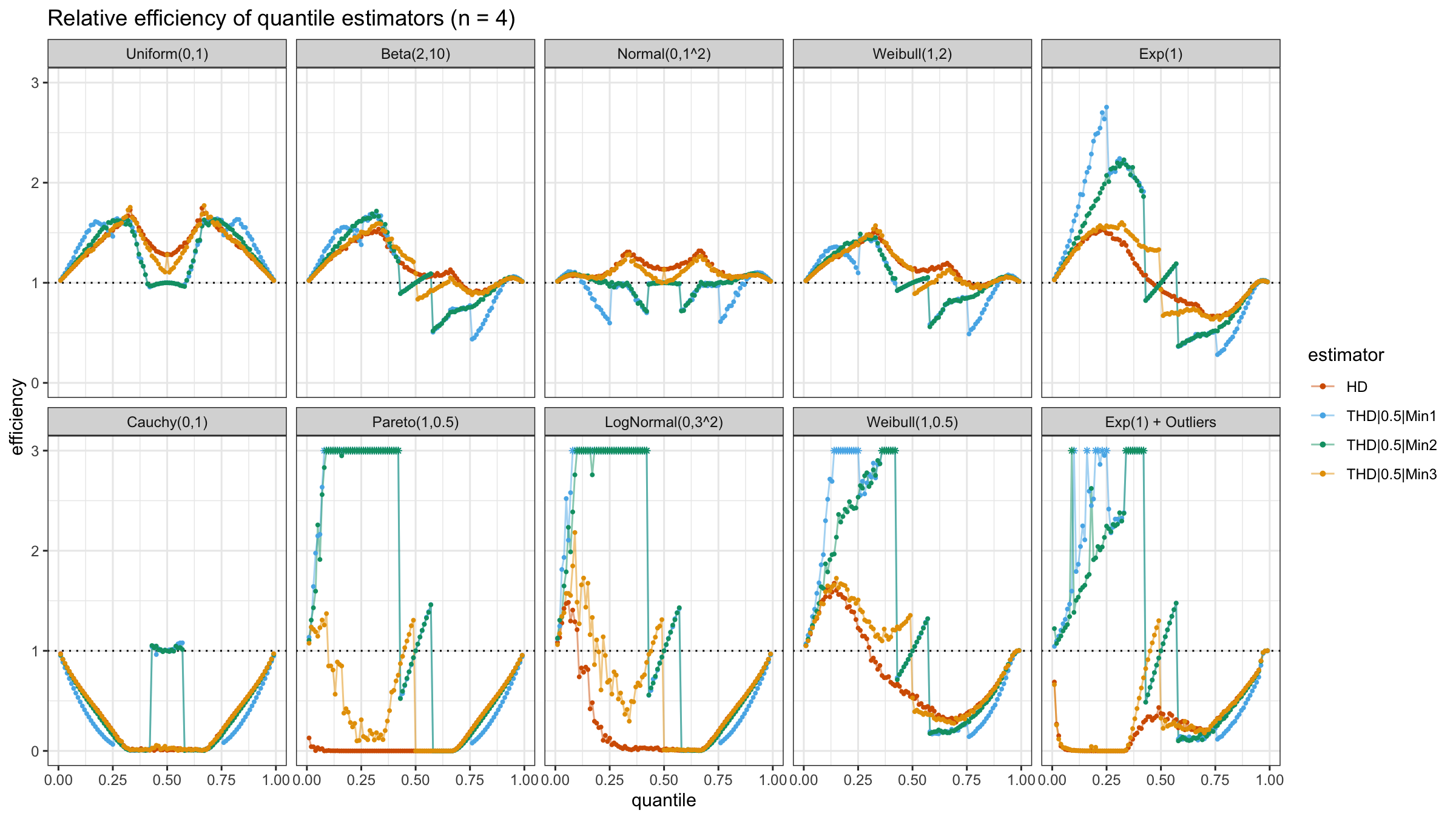
With N>3, all considered quantile estimators show different efficiency levels. We can see that all trimmed HDQEs work better than the classic HDQE in the heavy-tailed case and worse than the classic HDQE in the light-tailed case. However, there is a noticeable difference between different trimmed HDQEs on small light-tailed samples: THD|0.5|Min3 performs better than THD|0.5|Min1 and THD|0.5|Min2.

Conclusion

The choice of a quantile estimator is always a trade-off between robustness and efficiency. Specifying a lower bound for the number of target order statistics in the trimmed HDQE is one of the ways to control this trade-off. As we can see from the above simulations, such a trick could improve the statistical efficiency of trimmed HDQE in the light-tailed case by reducing the statistical efficiency in the heavy-tailed cases (meanwhile, it still keeps a better robustness level than the classic HDQE).