Optimal window of the trimmed Harrell-Davis quantile estimator, Part 1: Problems with the rectangular window

In the previous post, we have obtained a nice version of the trimmed Harrell-Davis quantile estimator which provides an opportunity to get a nice trade-off between robustness and statistical efficiency of quantile estimations. Unfortunately, it has a severe drawback. If we build a quantile-respectful density estimation based on the suggested estimator, we won’t get a smooth density function as in the case of the classic Harrell-Davis quantile estimator:

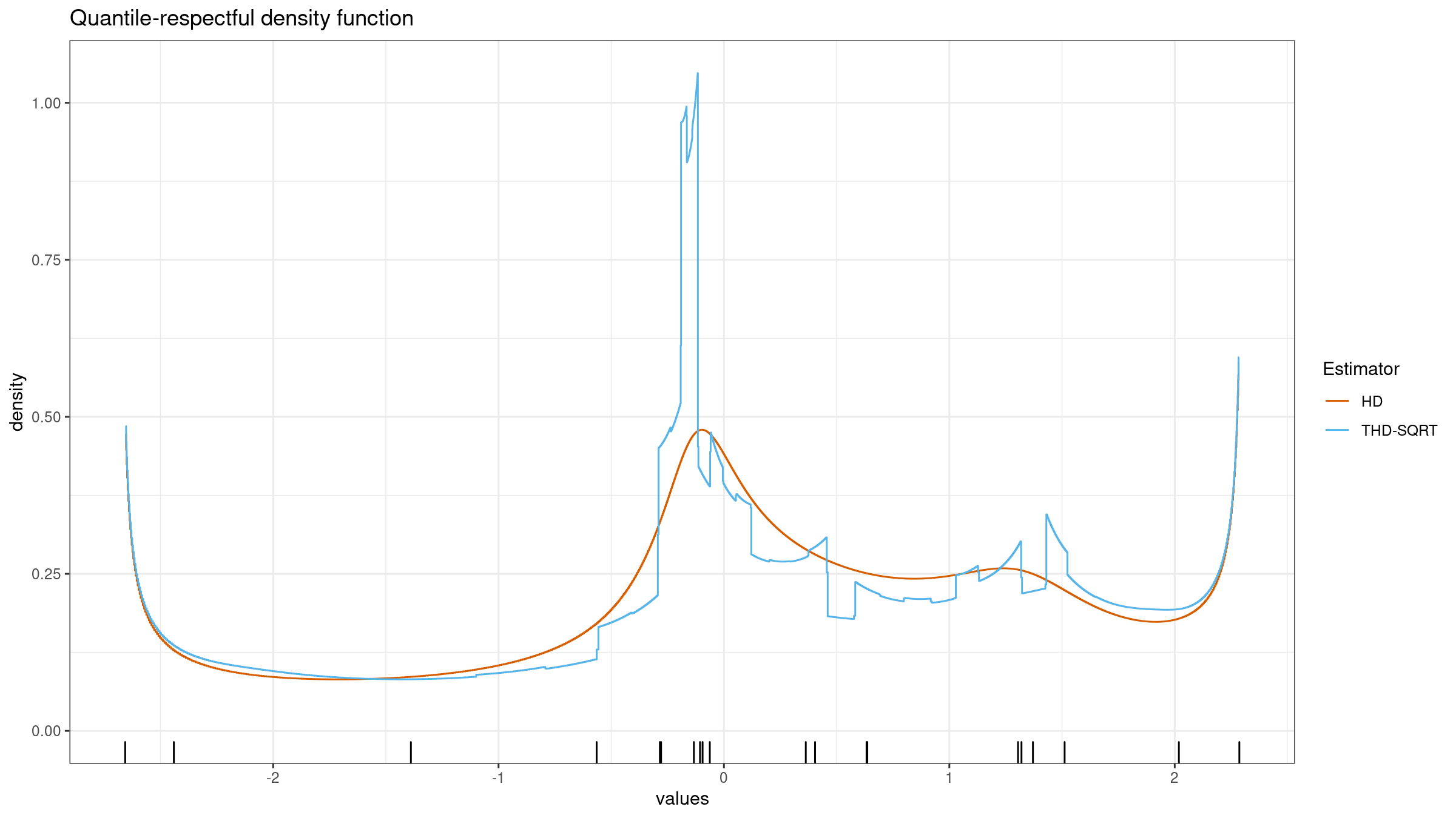
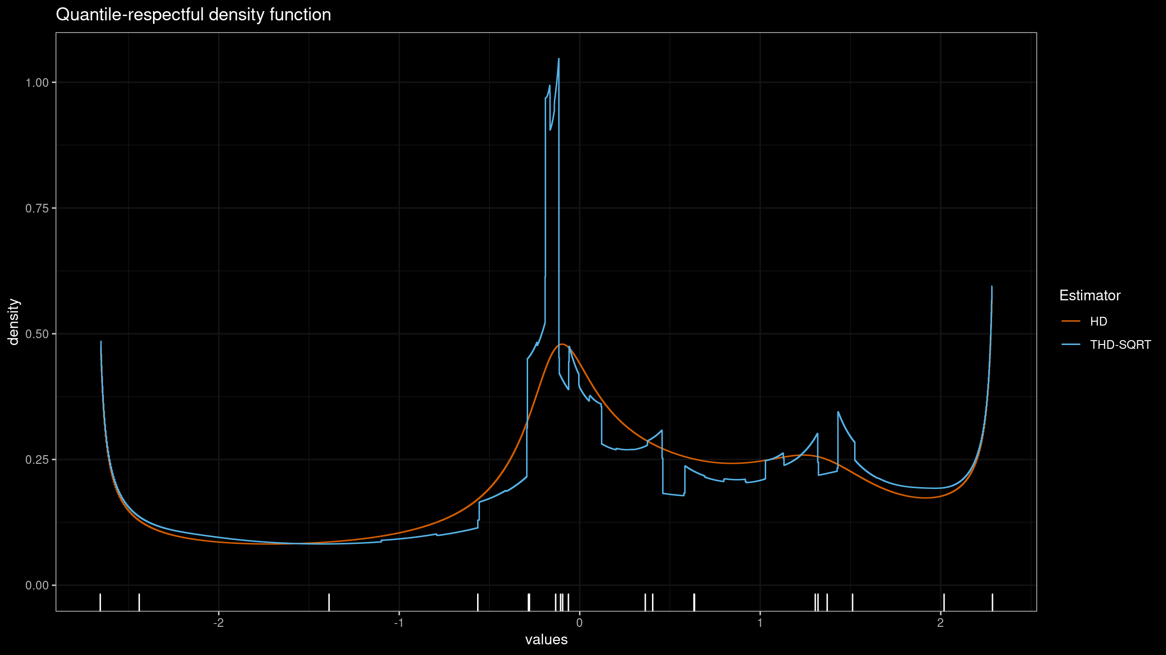
In this blog post series, we are going to find a way to improve the trimmed Harrell-Davis quantile estimator so that it gives a smooth density function and keeps its advantages in terms of robustness and statistical efficiency.

All posts from this series:

• Optimal window of the trimmed Harrell-Davis quantile estimator, Part 1: Problems with the rectangular window (2021-10-05)
• Optimal window of the trimmed Harrell-Davis quantile estimator, Part 2: Trying Planck-taper window (2021-10-12)

Trimmed Harrell-Davis quantile estimator

First of all, let’s recall the basic approach. We express the estimation of the $p^\textrm{th}$ quantile as a weighted sum of all order statistics:

$$ \begin{gather*} q_p = \sum_{i=1}^{n} W_{i} \cdot x_i,\\ W_{i} = F(r_i) - F(l_i),\\ l_i = (i - 1) / n, \quad r_i = i / n, \end{gather*} $$

where $F$ is a CDF function of a specific distribution. In the case of the Harrell-Davis quantile estimator, we use the Beta distribution. Thus, $F$ could be expressed via regularized incomplete beta function $I_x(\alpha, \beta)$:

$$ F_{\operatorname{HD}}(u) = I_u(\alpha, \beta), \quad \alpha = (n+1)p, \quad \beta = (n+1)(1 - p). $$

The Harrell-Davis quantile estimator has good statistical efficiency in the case of light-tailed distribution because it gathers all available information from the given samples. Unfortunately, this estimator is not robust. Indeed, a single corrupted sample element could corrupt all the quantile estimations.

That’s why we consider its trimmed version that aims to exclude extreme values from the summation. Thus, in the case of the trimmed Harrell-Davis quantile estimator, we use only a part of the Beta distribution inside the $[L,\, R]$ window. Thus, $F$ could be expressed as rescaled regularized incomplete beta function inside the given window:

$$ F_{\operatorname{THD}}(u) = \left\{ \begin{array}{lcrcllr} 0 & \textrm{for} & & & u & < & L, \\ (F_{\operatorname{HD}}(u) - F_{\operatorname{HD}}(L)) / (F_{\operatorname{HD}}(R) - F_{\operatorname{HD}}(L)) & \textrm{for} & L & \leq & u & \leq & R, \\ 1 & \textrm{for} & R & < & u. & & \end{array} \right. $$

The window is defined as the highest density interval of the given width. Using the window width as the estimator parameters, we can control the estimator robustness by setting a specific breakdown point value for the requested quantile.

Quantile-respectful density estimation

The quantile-respectful density estimation (QRDE) is a straightforward way of building a density function based on the given quantile estimation. Thus, it gives a density estimation that is consistent with the quantile values (unlike KDE). However, it requires a suitable quantile estimator. Traditional quantile estimator from the Hyndman-Fan classification (which are based on a linear combination of two order statistics) don’t provide a smooth density function. The Harrell-Davis quantile estimator provides a smooth density function, but it’s not robust. The trimmed Harrell-Davis quantile estimator has a customizable robustness level, but the corresponding density function has “steep steps:”

Our goal is to adjust the trimmed Harrell-Davis quantile estimator so that it has a smooth density function.

Representation via the rectangular window

To get a better understanding of these “steep steps,” we should take a look at another representation of the suggested quantile estimator. In order to do that, we should consider the probability density function that is used in the classic Harrell-Davis quantile estimator:

$$ f_{\operatorname{HD}}(x) = \frac{x^{\alpha - 1} (1 - x)^{\beta - 1}}{\operatorname{B}(\alpha, \beta)}. $$

If we split this function into n segments of equal width, the area under the curve in each segment will give us the weights $W_i$ of the sample order statistics:

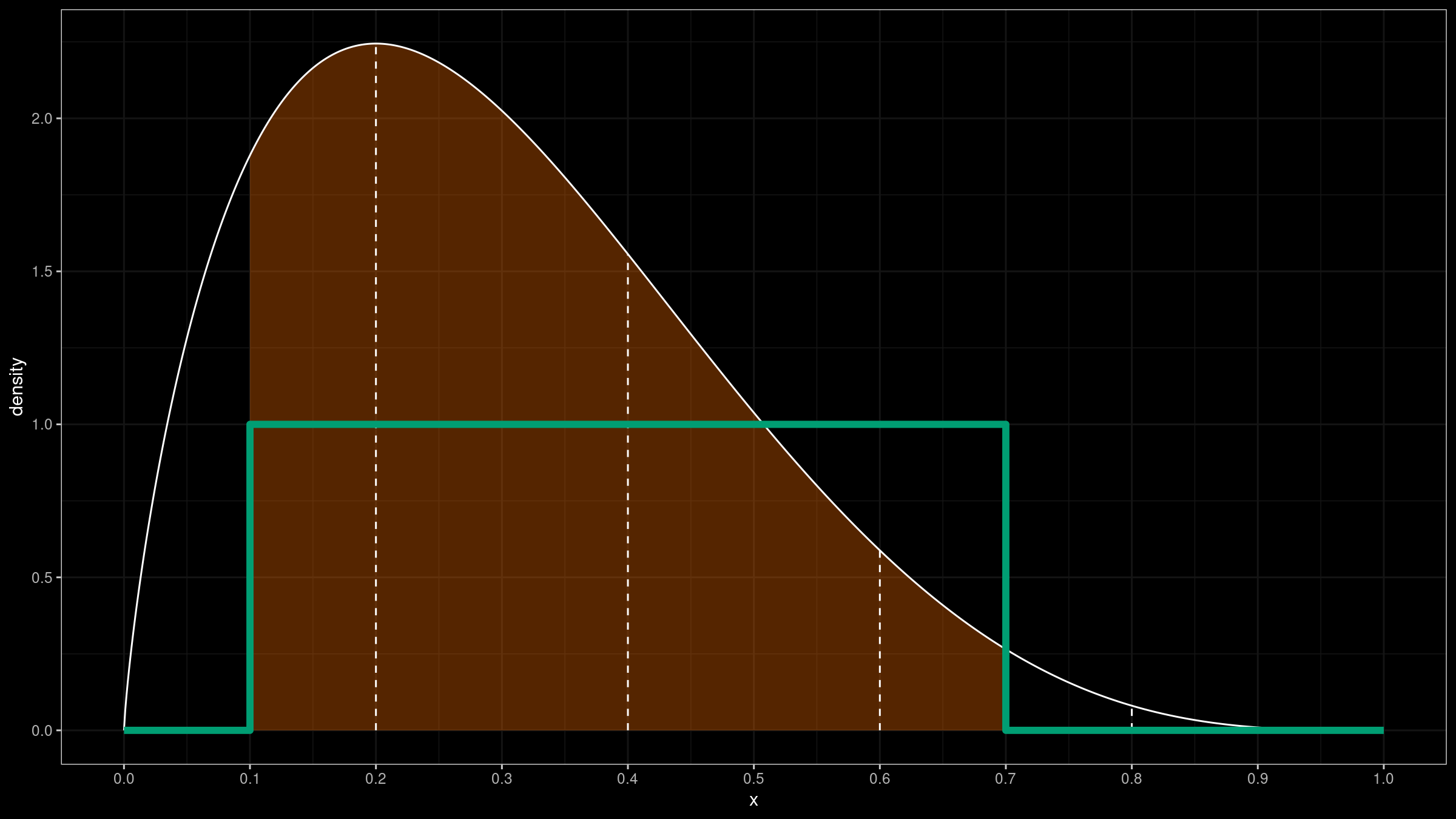
When we perform trimmification (and building a truncated distribution), we use only a part of $f_{\operatorname{HD}}(x)$:

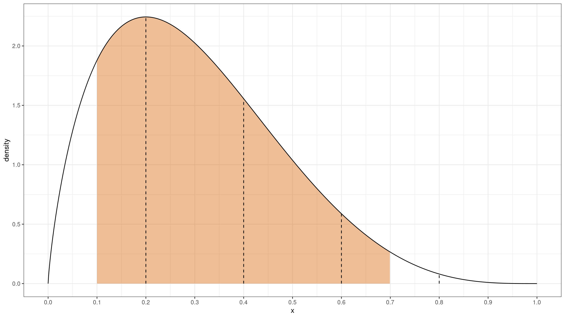
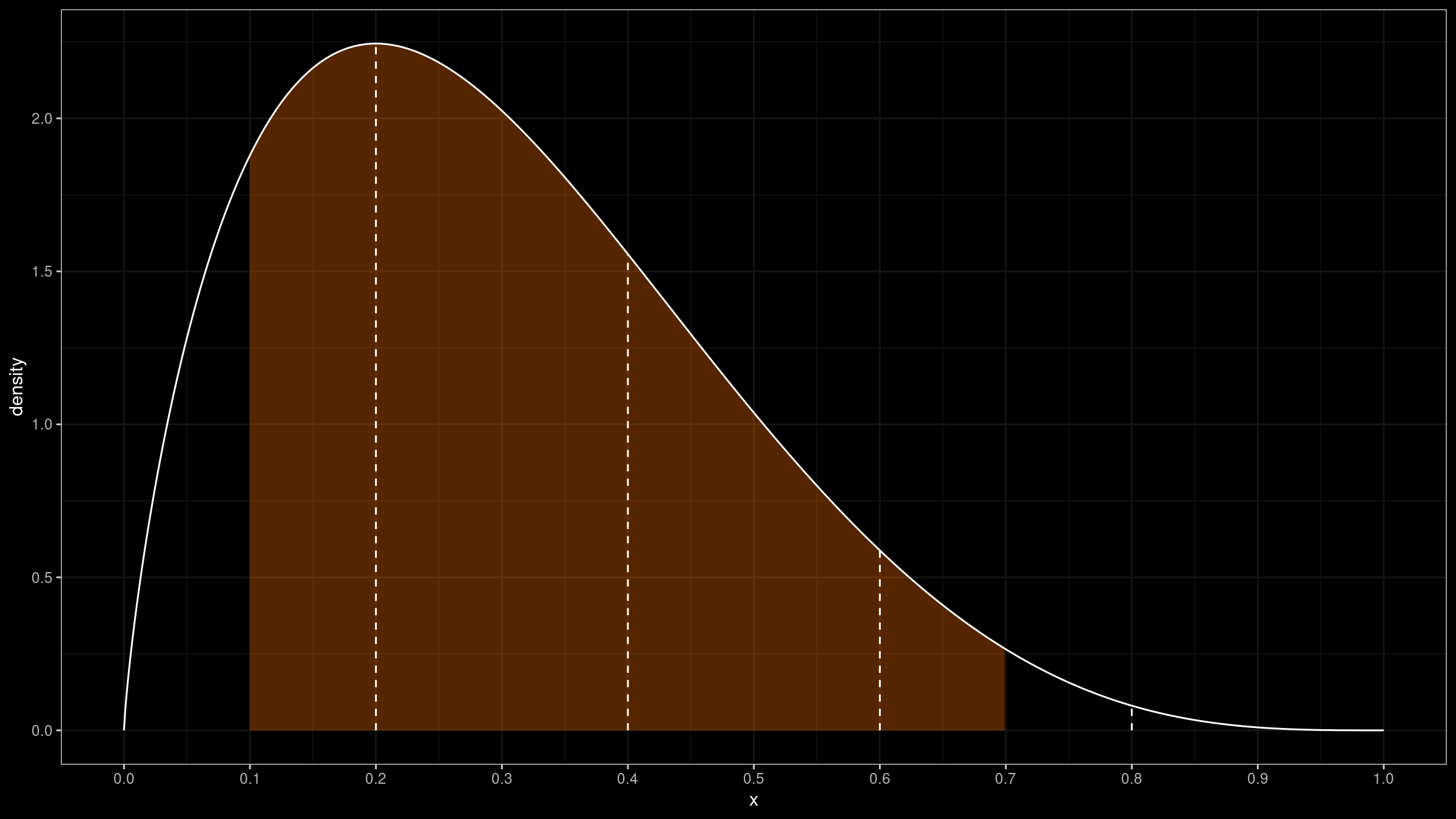
This operation could also be expressed using a rectangular window on $[L;R]$:

$$ f_{\operatorname{rw}}(x) = \begin{cases} 0, & \textrm{if }\, x < L,\\ 1, & \textrm{if }\, L \leq x \leq R,\\ 0, & \textrm{if }\, R < x.\\ \end{cases} $$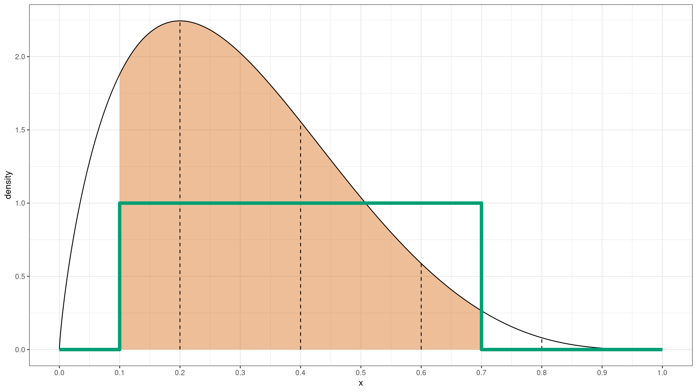

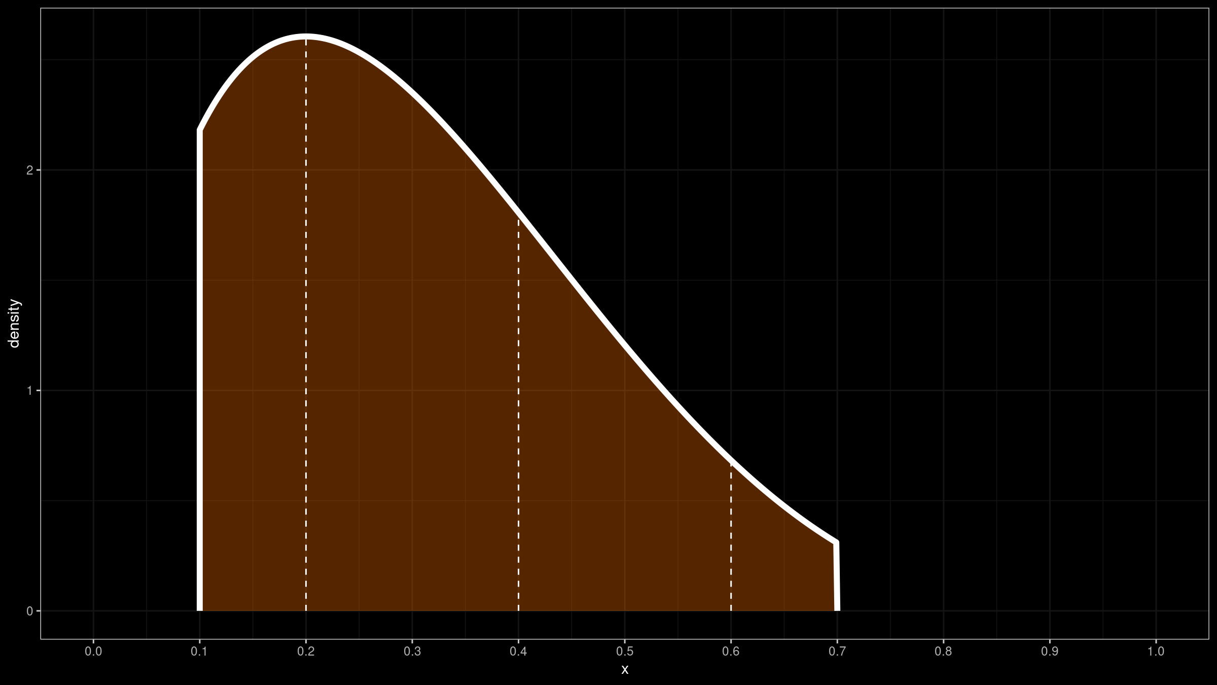
Thus, we could express the probability density function for the trimmed Harrell-Davis quantile estimator as a normalized multiplication of $f_{\operatorname{HD}}$ and $f_{\operatorname{rw}}$:

$$ f_{\operatorname{THD}}(x) = \dfrac{f_{\operatorname{HD}}(x) \cdot f_{\operatorname{rw}}(x)}{ \int_0^1 f_{\operatorname{HD}}(u) \cdot f_{\operatorname{rw}}(u) du} $$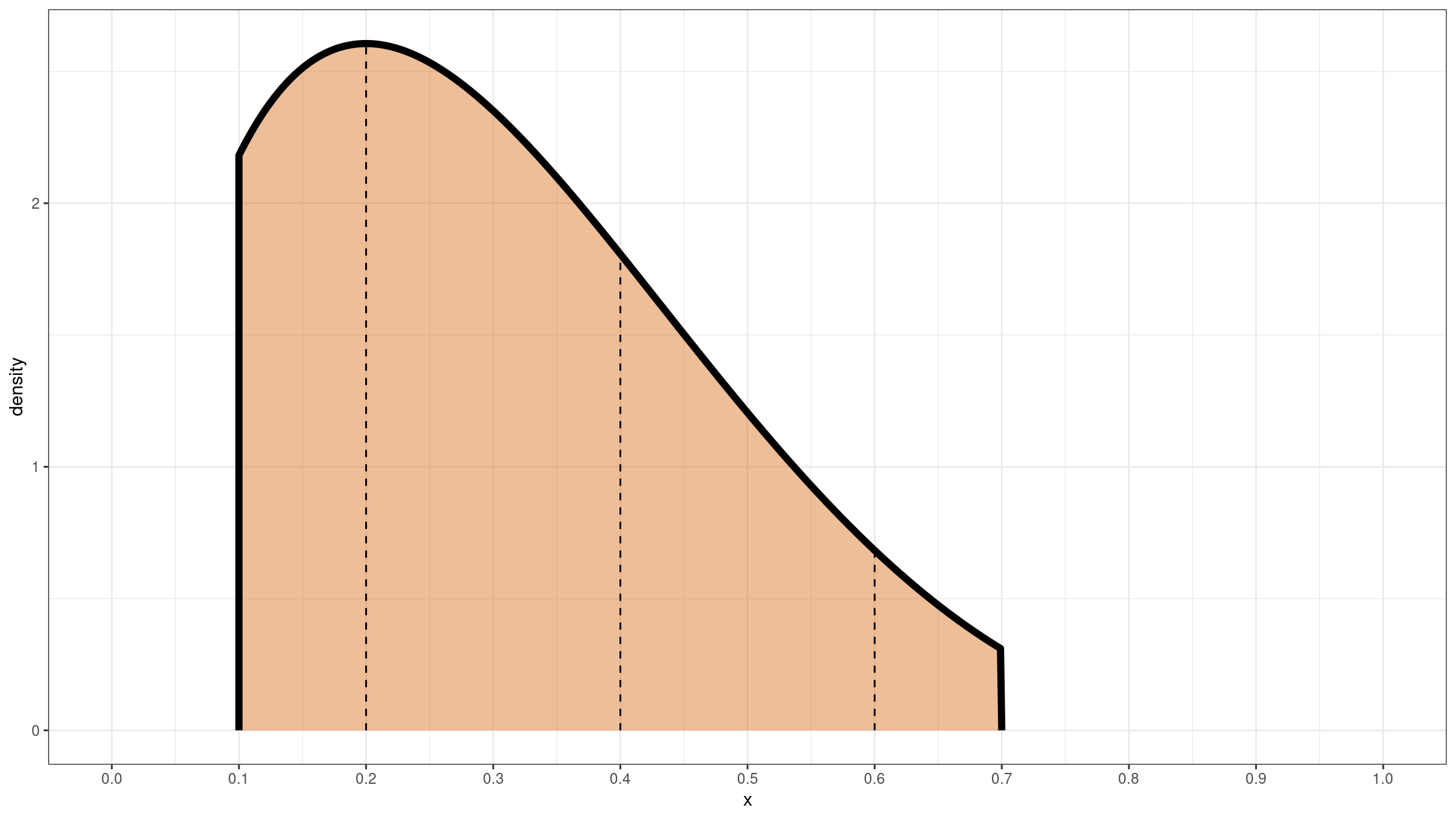

The corresponding cumulative density function could be easily found:

$$ F_{\operatorname{THD}}(x) = \int_0^x f_{\operatorname{THD}}(t) dt $$

Since $F_{\operatorname{THD}}(x)$ defines the weights $W_i$ of the sample order statistics, the discontinuities at points $L$ and $R$ spawn steps in the corresponding quantile-respectful density estimation.

Our next step is obvious: we should try to use smooth windows (e.g., Tukey window or Planck-taper window) instead of the rectangular window.