Optimal window of the trimmed Harrell-Davis quantile estimator, Part 2: Trying Planck-taper window

In the previous post, I discussed the problem of non-smooth quantile-respectful density estimation (QRDE) which is generated by the trimmed Harrell-Davis quantile estimator based on the highest density interval of the given width. I assumed that non-smoothness was caused by a non-smooth rectangular window which was used to build the truncated beta distribution. In this post, we are going to try another option: the Planck-taper window.

All posts from this series:

• Optimal window of the trimmed Harrell-Davis quantile estimator, Part 1: Problems with the rectangular window (October 5, 2021)
• Optimal window of the trimmed Harrell-Davis quantile estimator, Part 2: Trying Planck-taper window (October 12, 2021)

Planck-taper window

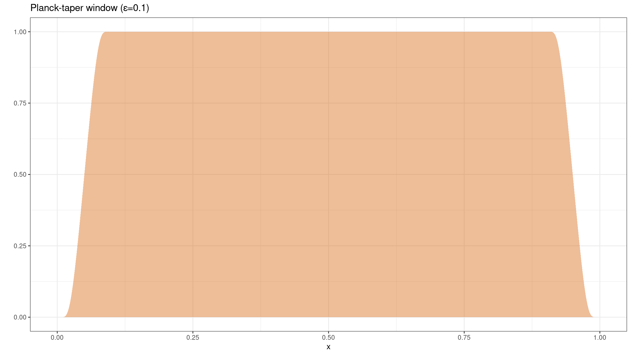
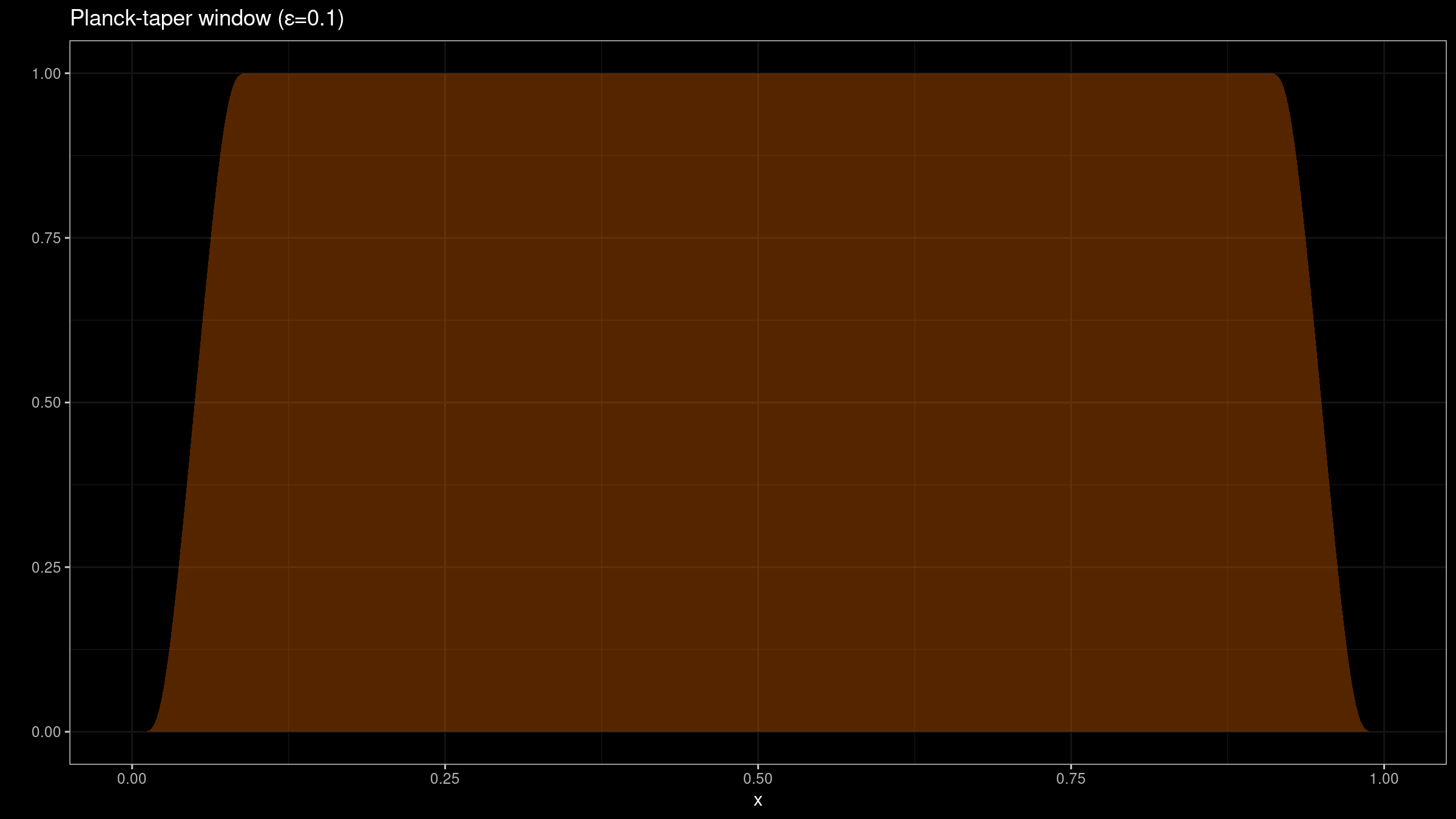
The Planck-taper window on $[0;1]$ could be expressed using the following function:

$$ h_\varepsilon(x) = \begin{cases} 0, & \textrm{for }\, x = 0,\\ \big( 1+e^{\frac{\varepsilon}{x} - \frac{\varepsilon}{\varepsilon - x}} \big)^{-1}, & \textrm{for }\, 0 < x < \varepsilon,\\ 1, & \textrm{for }\, \varepsilon \leq x \leq 1 - \varepsilon,\\ \big( 1+e^{\frac{\varepsilon}{1 - x} - \frac{\varepsilon}{\varepsilon - (1 - x)}} \big)^{-1}, & \textrm{for }\, 1 - \varepsilon < x < 1,\\ 0, & \textrm{for }\, x = 1.\\ \end{cases} $$

Here is an example of such function for $\varepsilon = 0.1$:

Planck-taper-powered trimmed Harrell-Davis quantile estimator

In the previous post, we discussed how to build a trimmed Harrell-Davis quantile estimator using a rectangular window. The suggested approach is based on the multiplication of the probability density function of the Beta distribution $f_{\operatorname{HD}}$ (which is used in the classic Harrell-Davis quantile estimator) and the rectangular window $f_{\operatorname{rw}}$:

$$ f_{\operatorname{HD}}(x) = \frac{x^{\alpha - 1} (1 - x)^{\beta - 1}}{\operatorname{B}(\alpha, \beta)}. $$ $$ f_{\operatorname{rw}}(x) = \begin{cases} 0, & \textrm{if }\, x < L,\\ 1, & \textrm{if }\, L \leq x \leq R,\\ 0, & \textrm{if }\, R < x.\\ \end{cases} $$ $$ f_{\operatorname{THD/rw}}(x) = \dfrac{f_{\operatorname{HD}}(x) \cdot f_{\operatorname{rw}}(x)}{ \int_0^1 f_{\operatorname{HD}}(u) \cdot f_{\operatorname{rw}}(u) du} $$ $$ F_{\operatorname{THD/rw}}(x) = \int_0^x f_{\operatorname{THD/rw}}(t) dt $$

This time, we are going to use the same procedure for the following multiplier function based on the Planck-taper window:

$$ f_{\operatorname{ptw}}(x) = \begin{cases} 0, & \textrm{if }\, x < L,\\ h_\varepsilon((x - L) / (R - L)), & \textrm{if }\, L \leq x \leq R,\\ 0, & \textrm{if }\, R < x.\\ \end{cases} $$ $$ f_{\operatorname{THD/ptw}}(x) = \dfrac{f_{\operatorname{HD}}(x) \cdot f_{\operatorname{ptw}}(x)}{ \int_0^1 f_{\operatorname{HD}}(u) \cdot f_{\operatorname{ptw}}(u) du} $$ $$ F_{\operatorname{THD/ptw}}(x) = \int_0^x f_{\operatorname{THD/ptw}}(t) dt $$

Simulation results

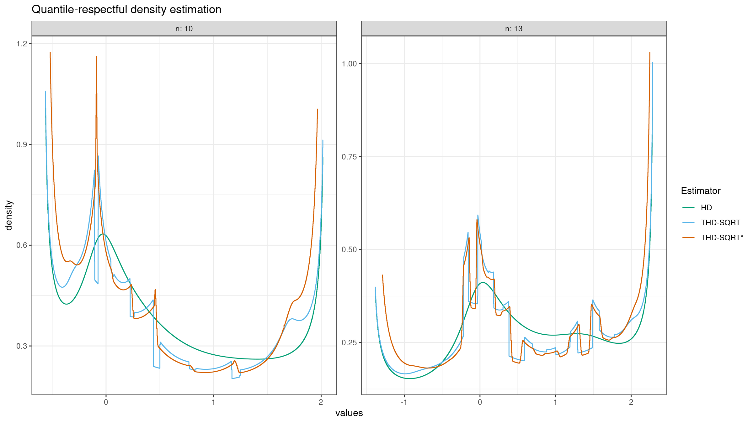
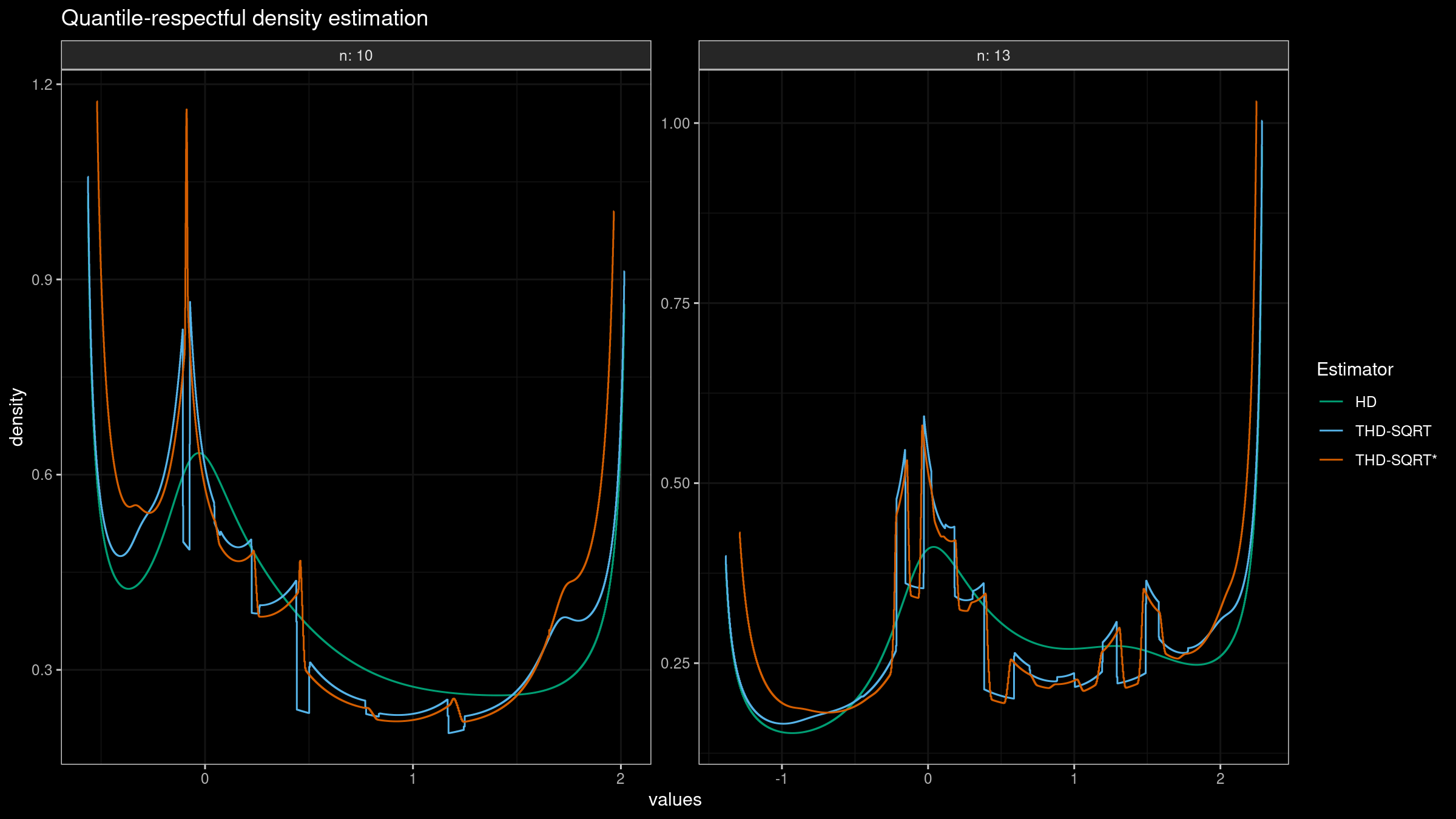
I have tried multiple combinations of sample sizes, $\varepsilon$ values, and trimming percentage values. In most cases, the Planck-taper-powered estimator gives quantile-respectful density estimation that a little bit smoother than the estimation in the rectangular window case.

(Quantile estimator based on the Planck-taper window is denoted as THD-SQRT*)

Discussion

It seems that we can’t obtain smooth density estimation using trimmed quantile estimators regardless of the window form. Here is the intuition behind the density estimation discontinuous points (that looks like steps). Imagine that we slowly change the probability $p$ of the target quantile from $0$ to $1$ and build the corresponding density function values. Each $p$ value gives us the $[L;R]$ interval which defines the set of order statistics that are actually used to build the quantile estimation. While we change $p$ from $0$ to $1$, we also change $[L;R]$ from $[0;w]$ to $[1-w;1]$ where $w$ is the interval width. When the $[L;R]$ interval crosses a border between two order statistics, it starts to cover another sample element. If the gap between these two order statistics is huge, we could observe a density functions step regardless of the smoothness of $W_i(p)$. Using different window functions, we could improve smoothness a little bit, but it seems to be impossible to get rid of steps completely. Apparently, this is the price of estimator robustness.