Optimal threshold of the trimmed Harrell-Davis quantile estimator

The traditional quantile estimators (which are based on 1 or 2 order statistics) have great robustness. However, the statistical efficiency of these estimators is not so great. The Harrell-Davis quantile estimator has much better efficiency (at least in the light-tailed case), but it’s not robust (because it calculates a weighted sum of all sample values). I already wrote a post about trimmed Harrell-Davis quantile estimator: this approach suggest dropping some of the low-weight sample values to improve robustness (keeping good statistical efficiency). I also perform a numerical simulations that compare efficiency of the original Harrell-Davis quantile estimator against its trimmed and winsorized modifications. It’s time to discuss how to choose the optimal trimming threshold and how it affects the estimator efficiency.

Simulation design

The relative efficiency value depends on five parameters:

• Target quantile estimator
• Baseline quantile estimator
• Estimated quantile $p$
• Sample size $n$
• Distribution

As target quantile estimators, we use the trimmed Harrell-Davis quantile estimators with different trimming percentage values.

The conventional baseline quantile estimator in such simulations is the traditional quantile estimator that is defined as a linear combination of two subsequent order statistics. To be more specific, we are going to use the Type 7 quantile estimator from the Hyndman-Fan classification or HF7 (hyndman1996). It can be expressed as follows (assuming one-based indexing):

$$ Q_{HF7}(p) = x_{(\lfloor h \rfloor)}+(h-\lfloor h \rfloor)(x_{(\lfloor h \rfloor+1)})-x_{(\lfloor h \rfloor)},\quad h = (n-1)p+1. $$

Thus, we are going to estimate the relative efficiency of the trimmed Harrell-Davis quantile estimator with different percentage values against the traditional quantile estimator HF7. For the $p^\textrm{th}$ quantile, the classic relative efficiency can be calculated as the ratio of the estimator mean squared errors ($\textrm{MSE}$):

$$ \textrm{Efficiency}(p) = \dfrac{\textrm{MSE}(Q_{HF7}, p)}{\textrm{MSE}(Q_{HD}, p)} = \dfrac{\operatorname{E}[(Q_{HF7}(p) - \theta(p))^2]}{\operatorname{E}[(Q_{HD}(p) - \theta(p))^2]} $$

where $\theta(p)$ is the true value of the $p^\textrm{th}$ quantile. The $\textrm{MSE}$ value depends on the sample size $n$, so it should be calculated independently for each sample size value.

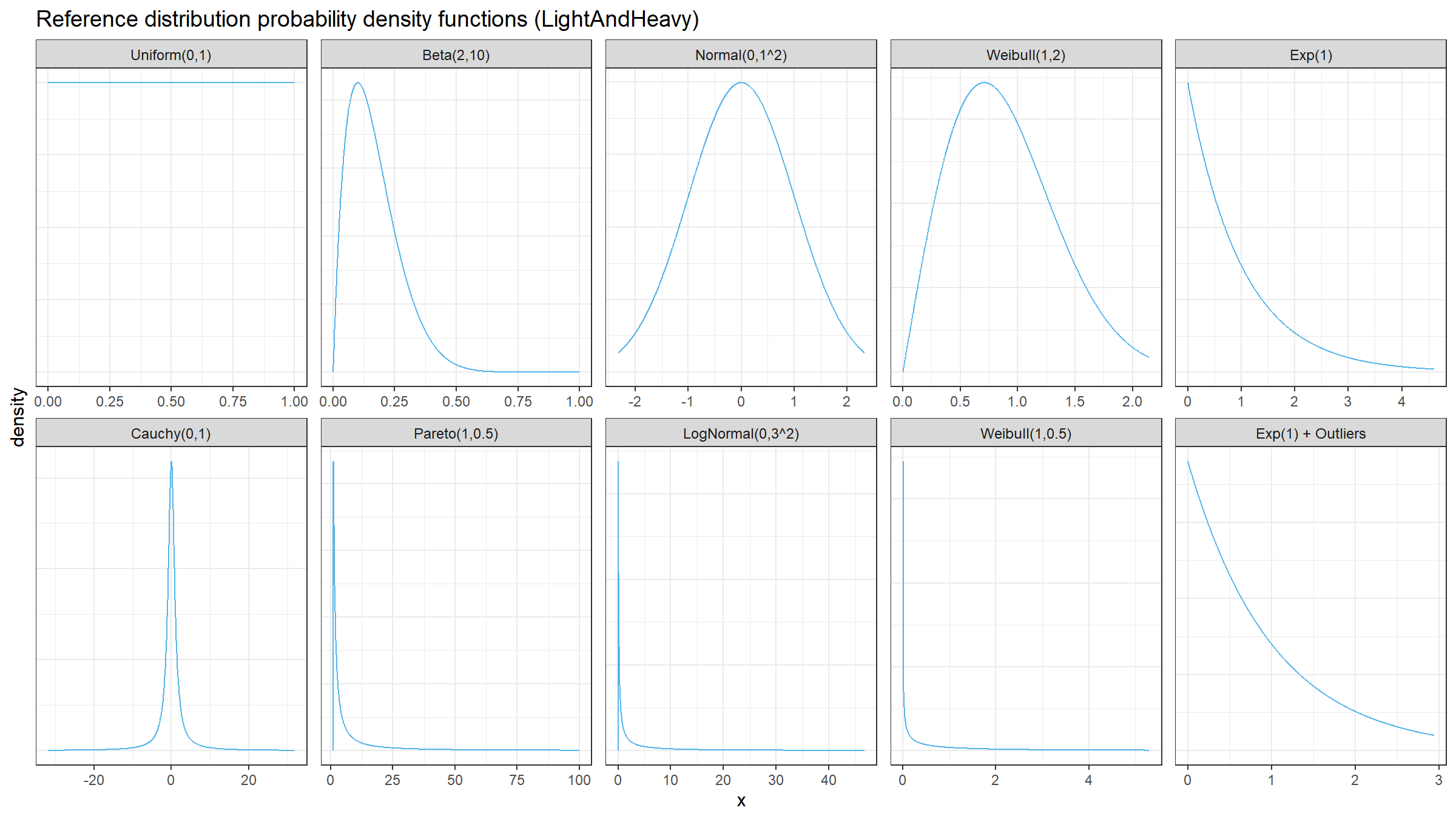
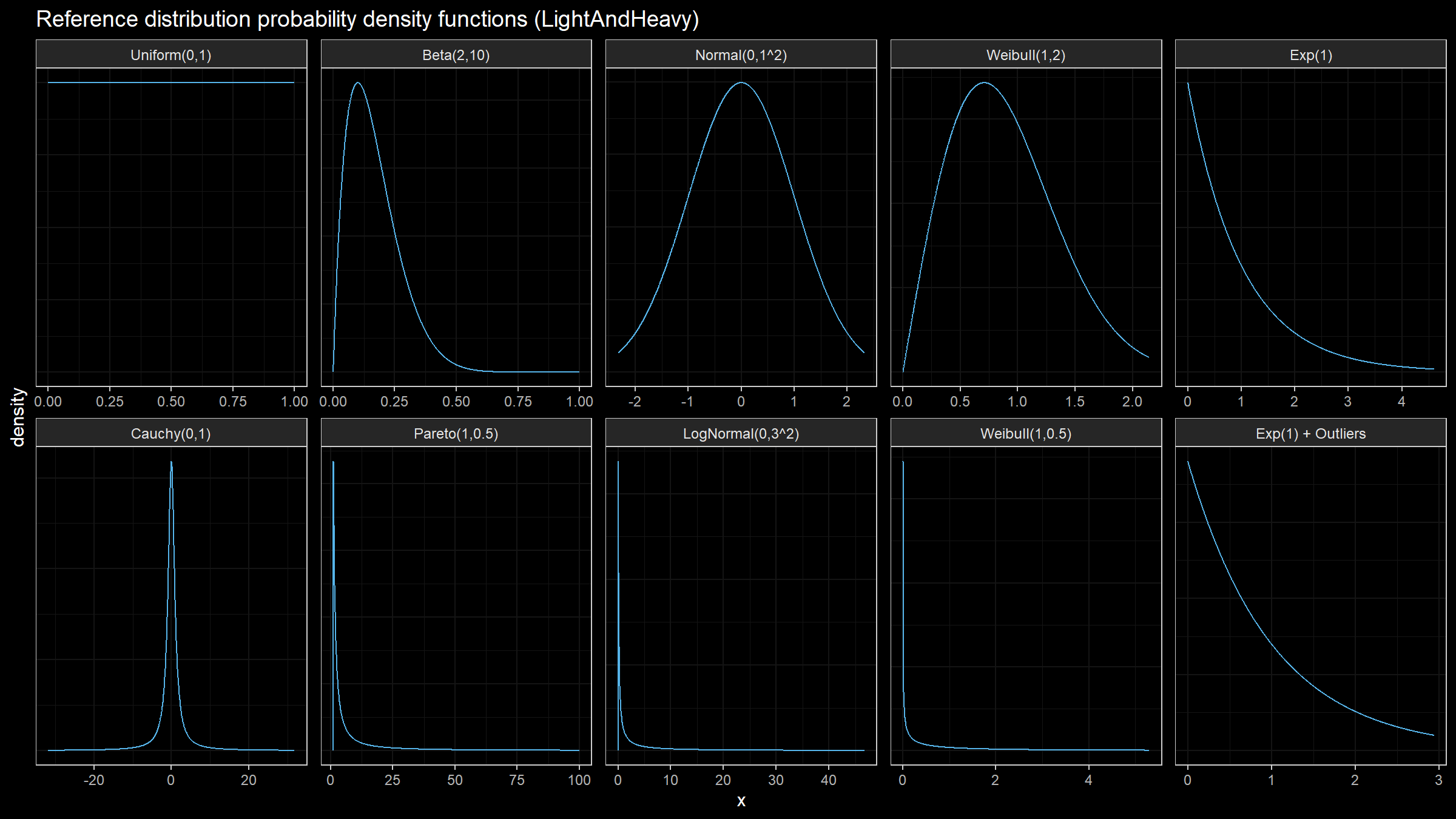
Finally, we should choose the distributions for sample generation. I decided to choose 5 light-tailed distributions and 5 heavy-tailed distributions

distribution	description
U(0,1)	Uniform distribution on [0;1]
Beta(2,10)	Beta distribution with a=2, b=10
N(0,1^2)	Normal distribution with mu=0, sigma=1
Weibull(1,2)	Weibull distribution with scale=1, shape=2
Exp(1)	Exponential distribution
Cauchy(0,1)	Cauchy distribution with location=0, scale=1
Pareto(1, 0.5)	Pareto distribution with xm=1, alpha=0.5
LogNormal(0,3^2)	Log-normal distribution with mu=0, sigma=3
Weibull(1,2)	Weibull distribution with scale=1, shape=0.5
Exp(1) + Outliers	95% of exponential distribution with rate=1 and 5% of uniform distribution on [0;10000]

Here are the probability density functions of these distributions:

For each distribution, we are going to do the following:

• Enumerate all the percentiles and calculate the true percentile value $\theta(p)$ for each distribution
• Enumerate different sample sizes (from 3 to 40)
• Generate a bunch of random samples, estimate the percentile values using all estimators, calculate the relative efficiency of all target quantile estimators quantile estimator.

Simulation results

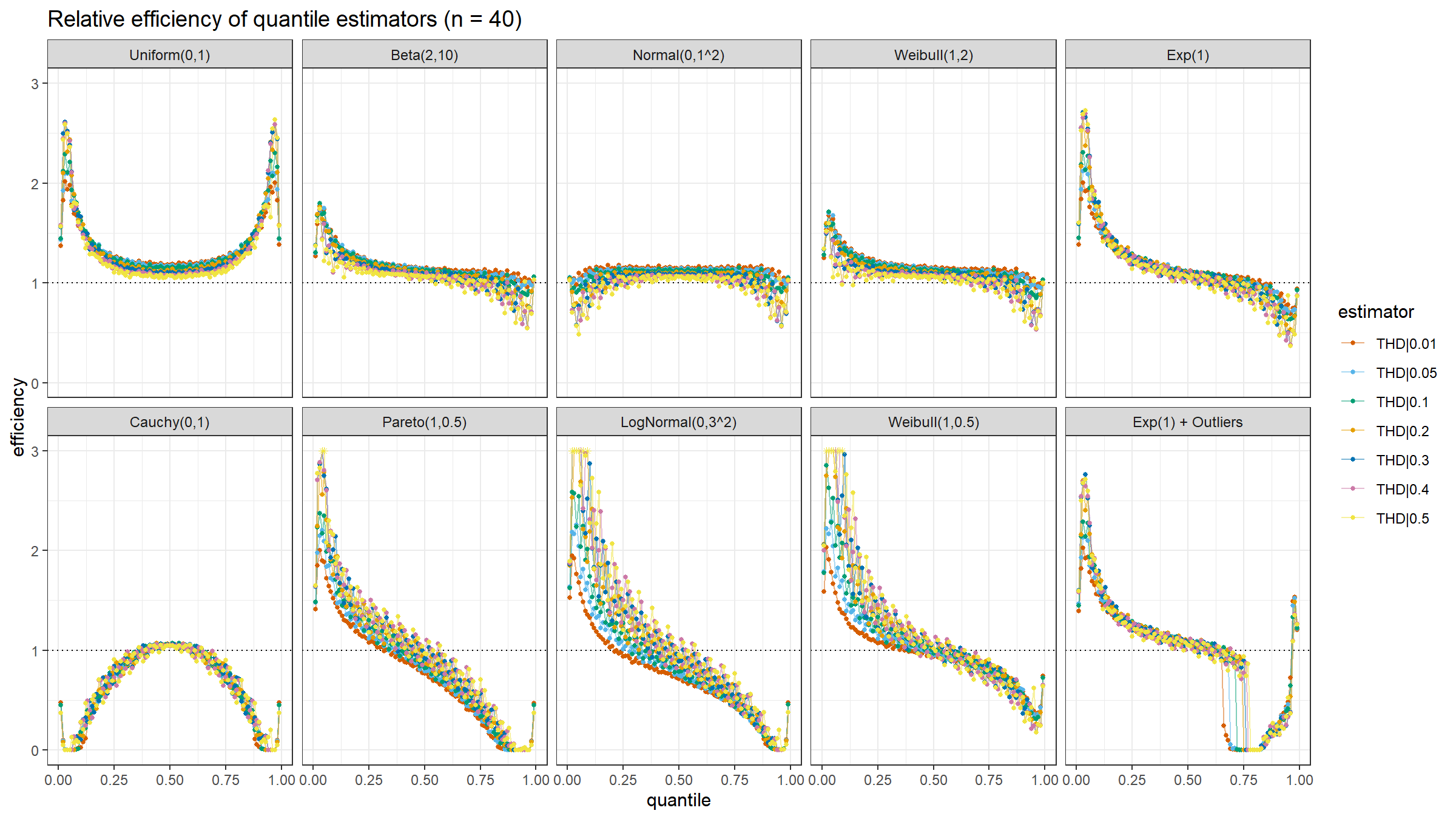
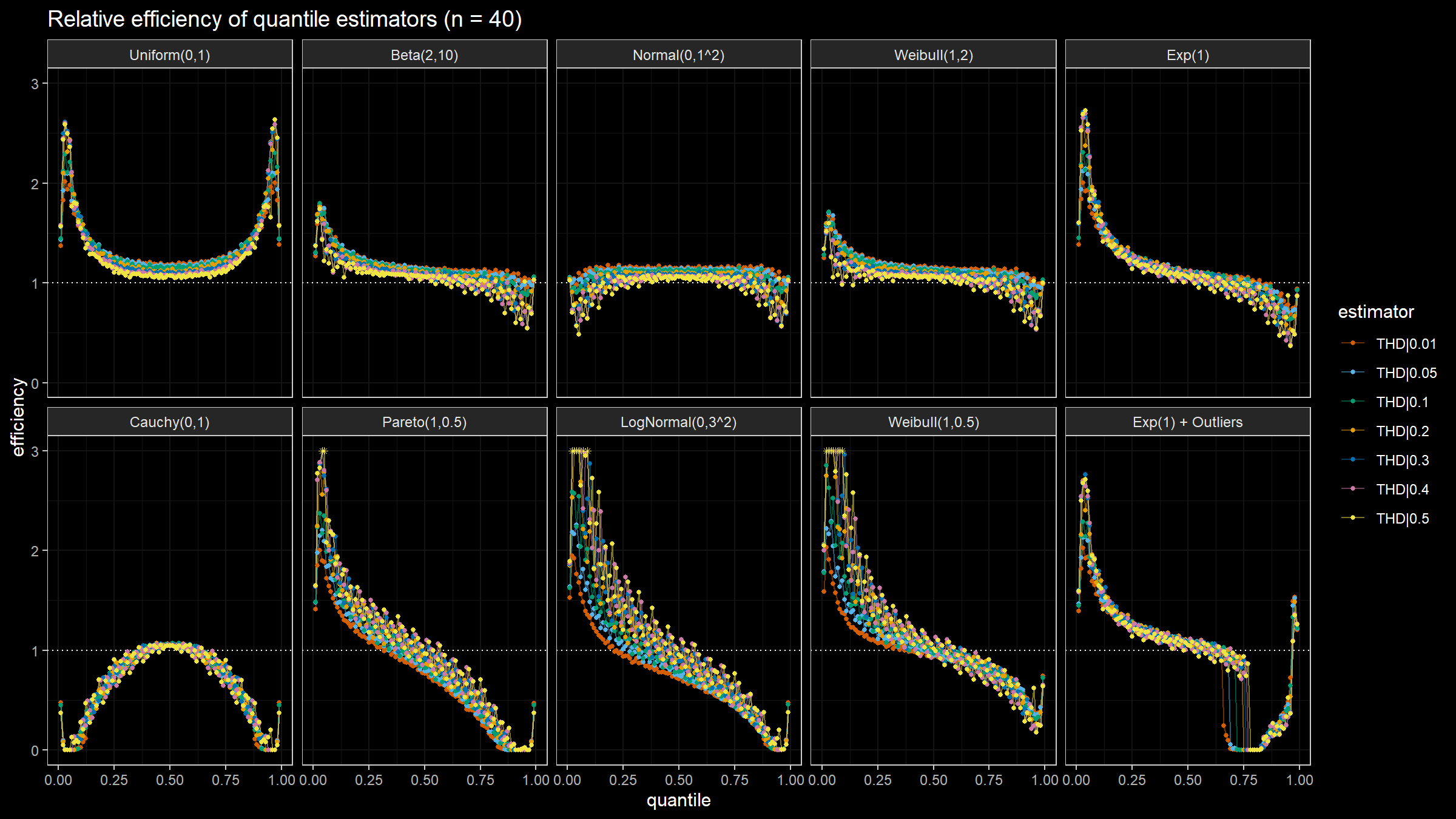
Here are the animated results of the simulation:

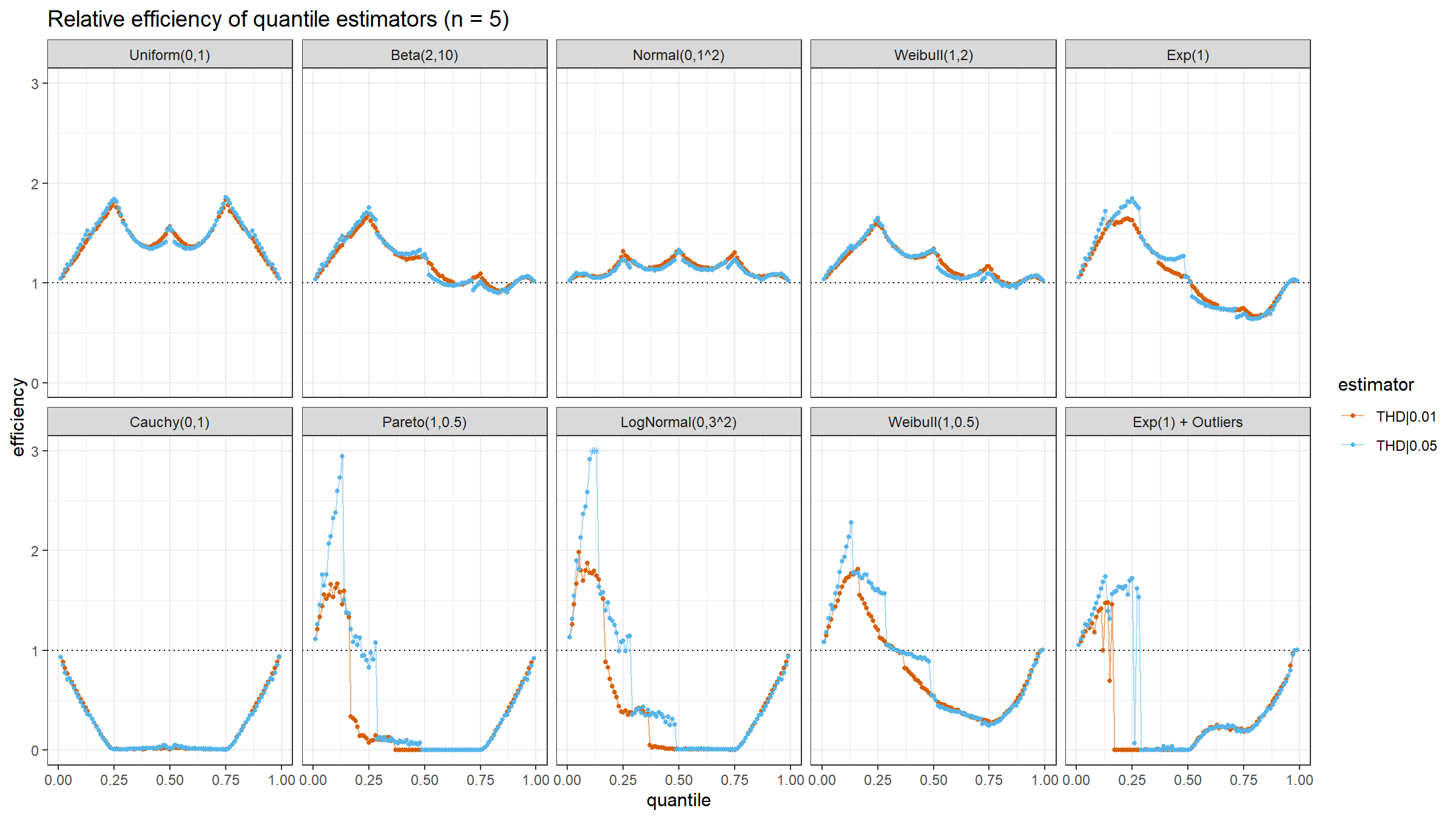
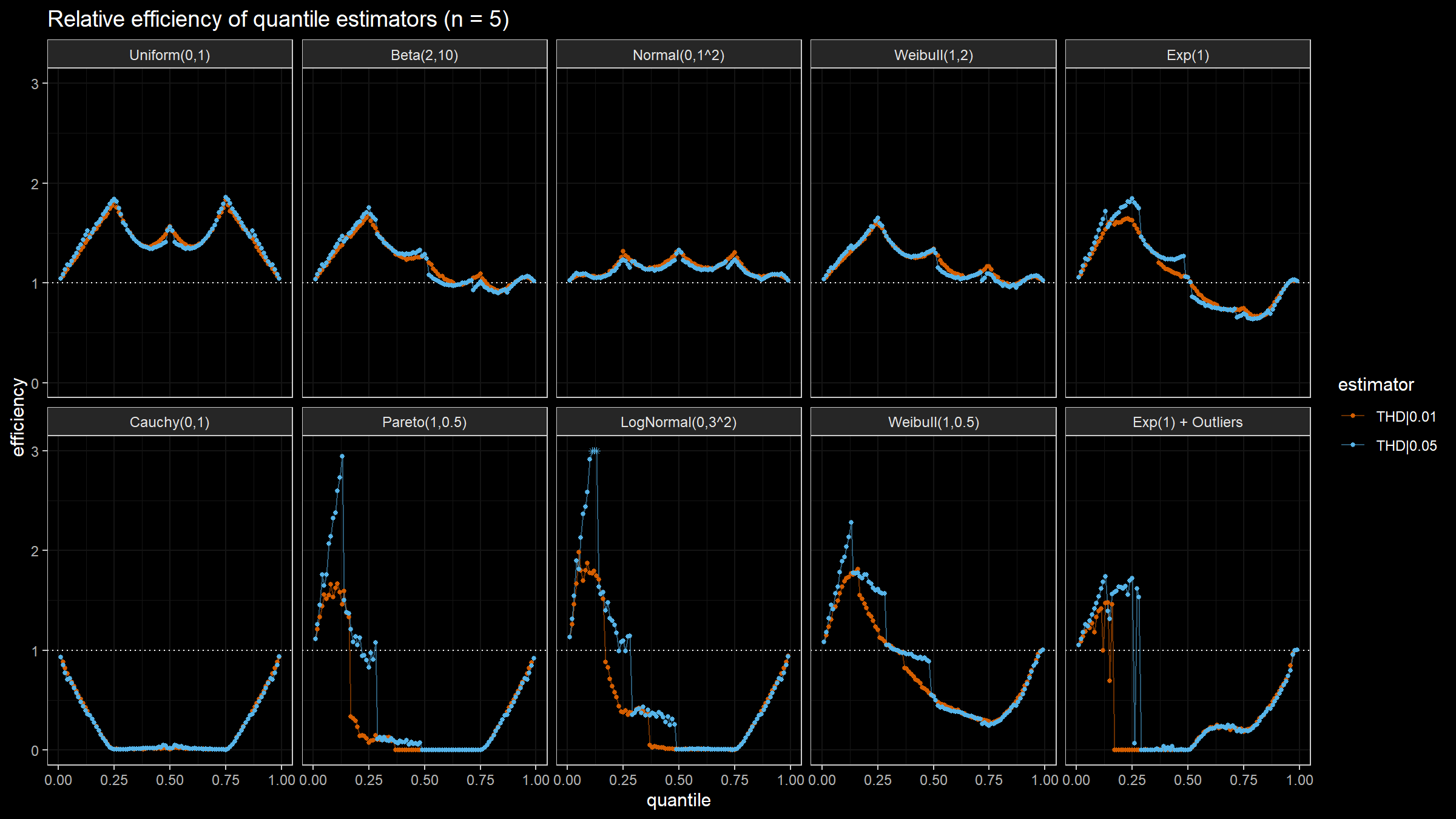
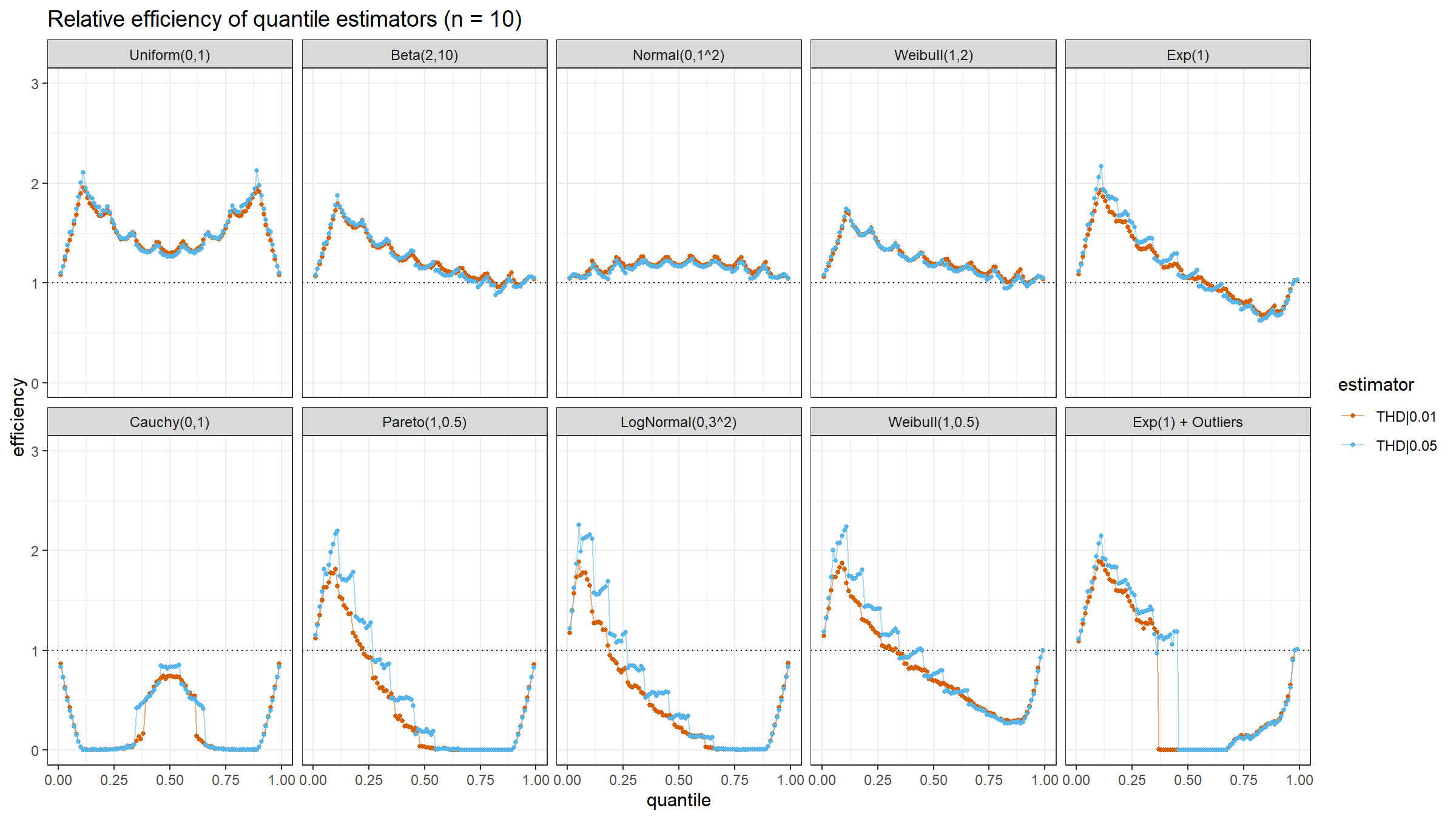
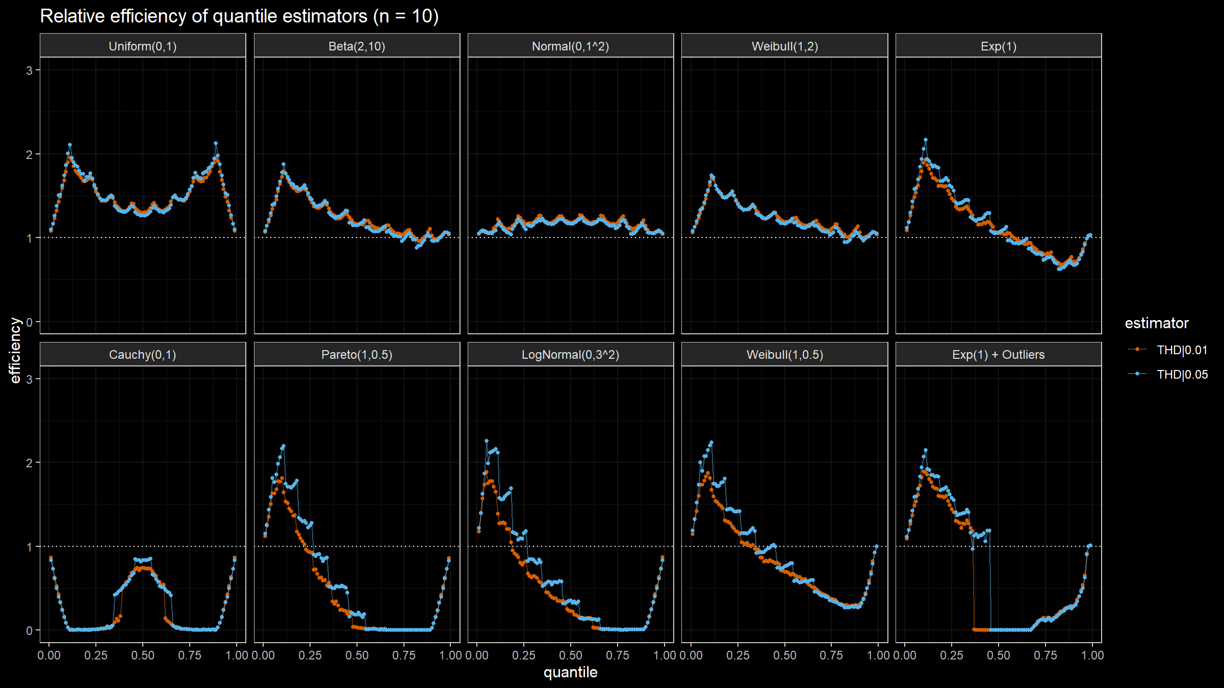
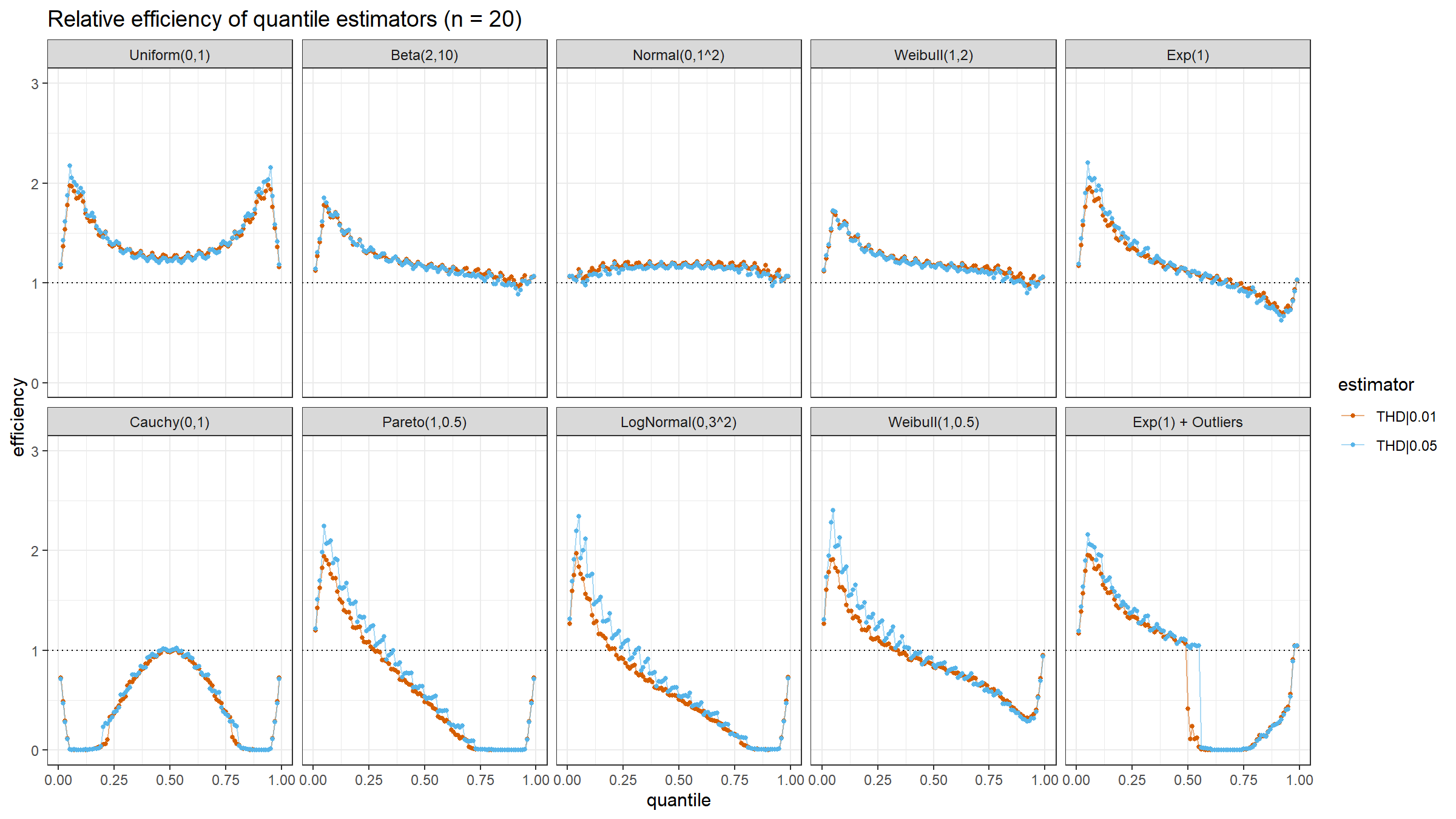
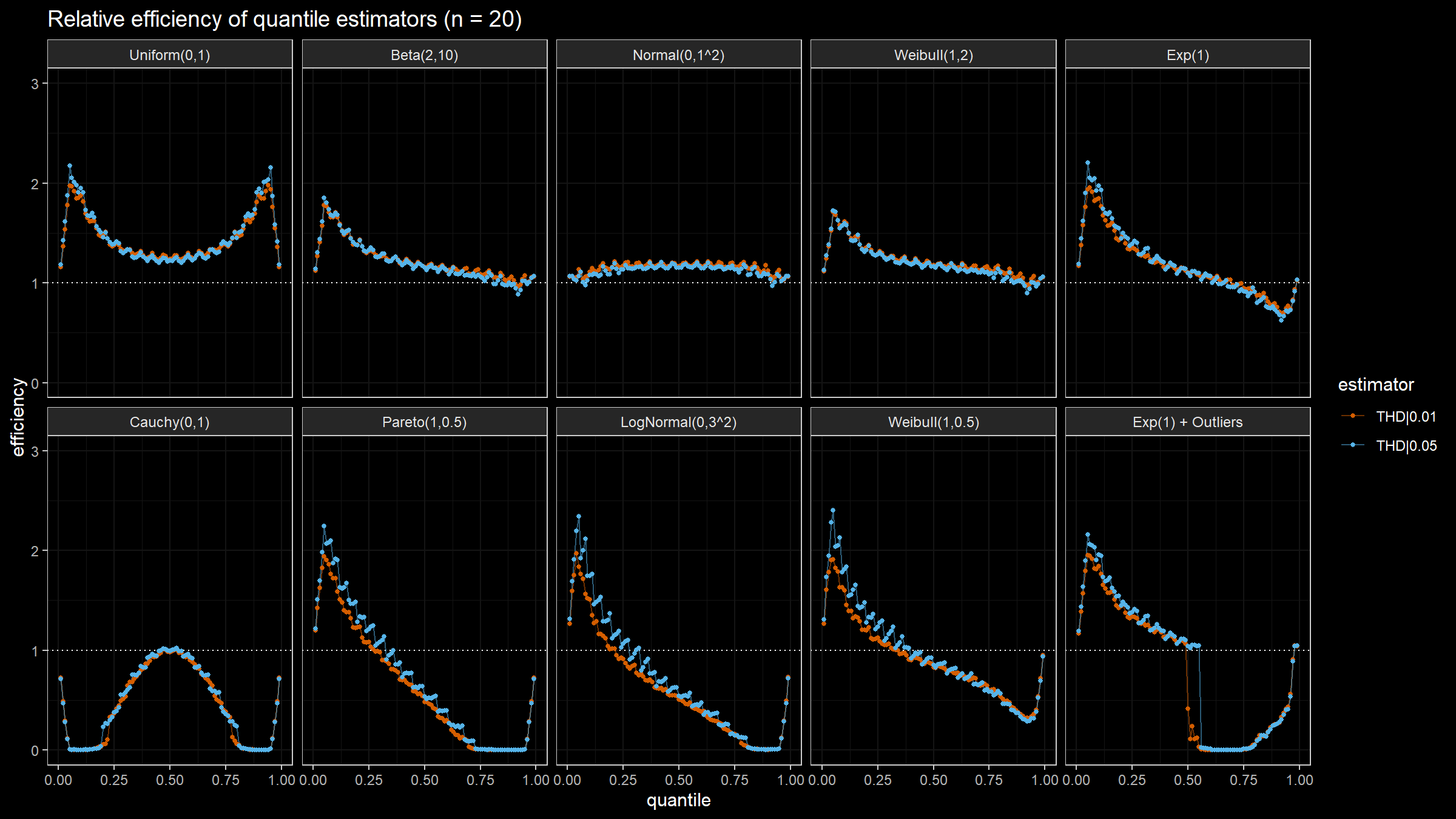
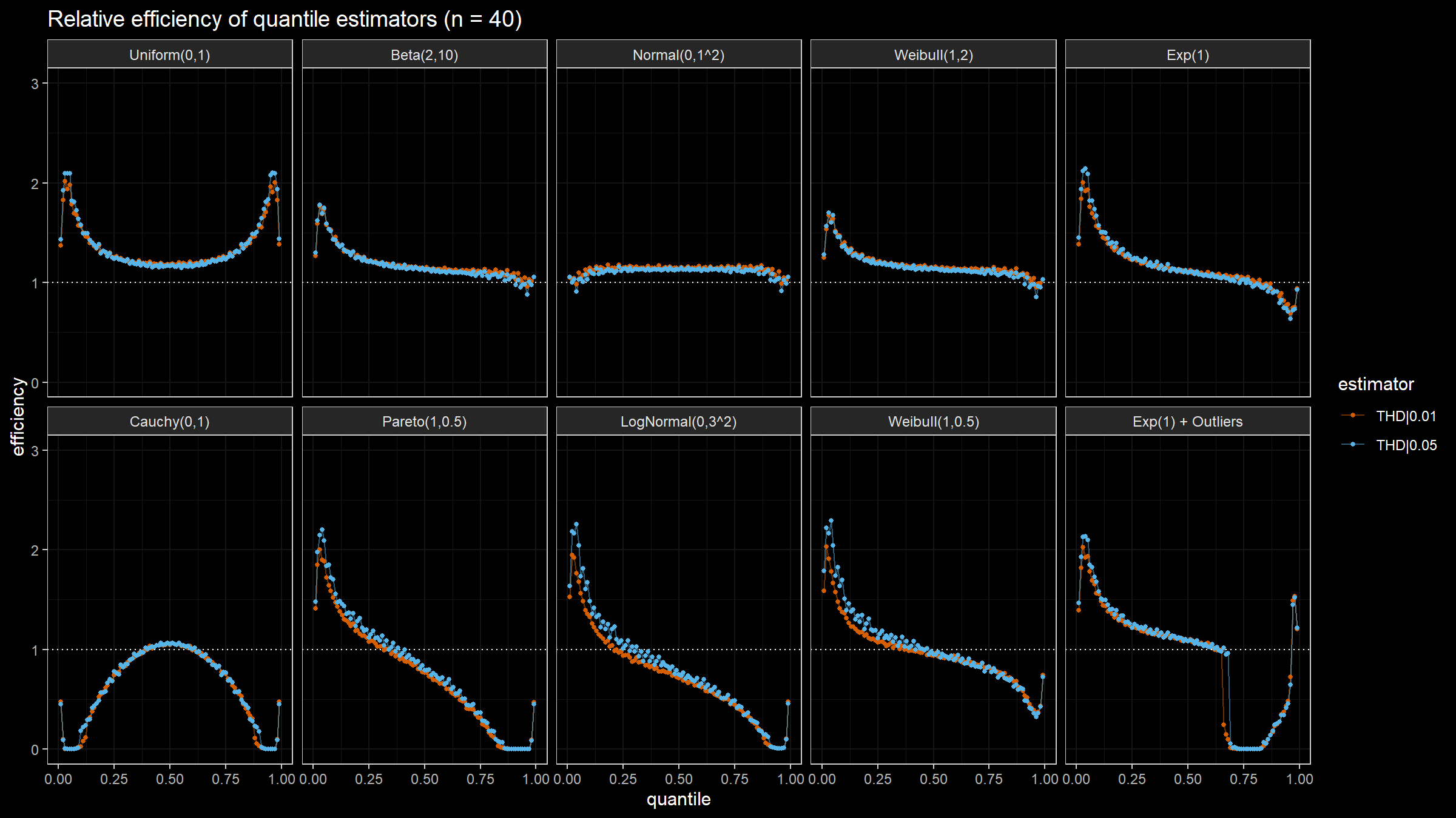
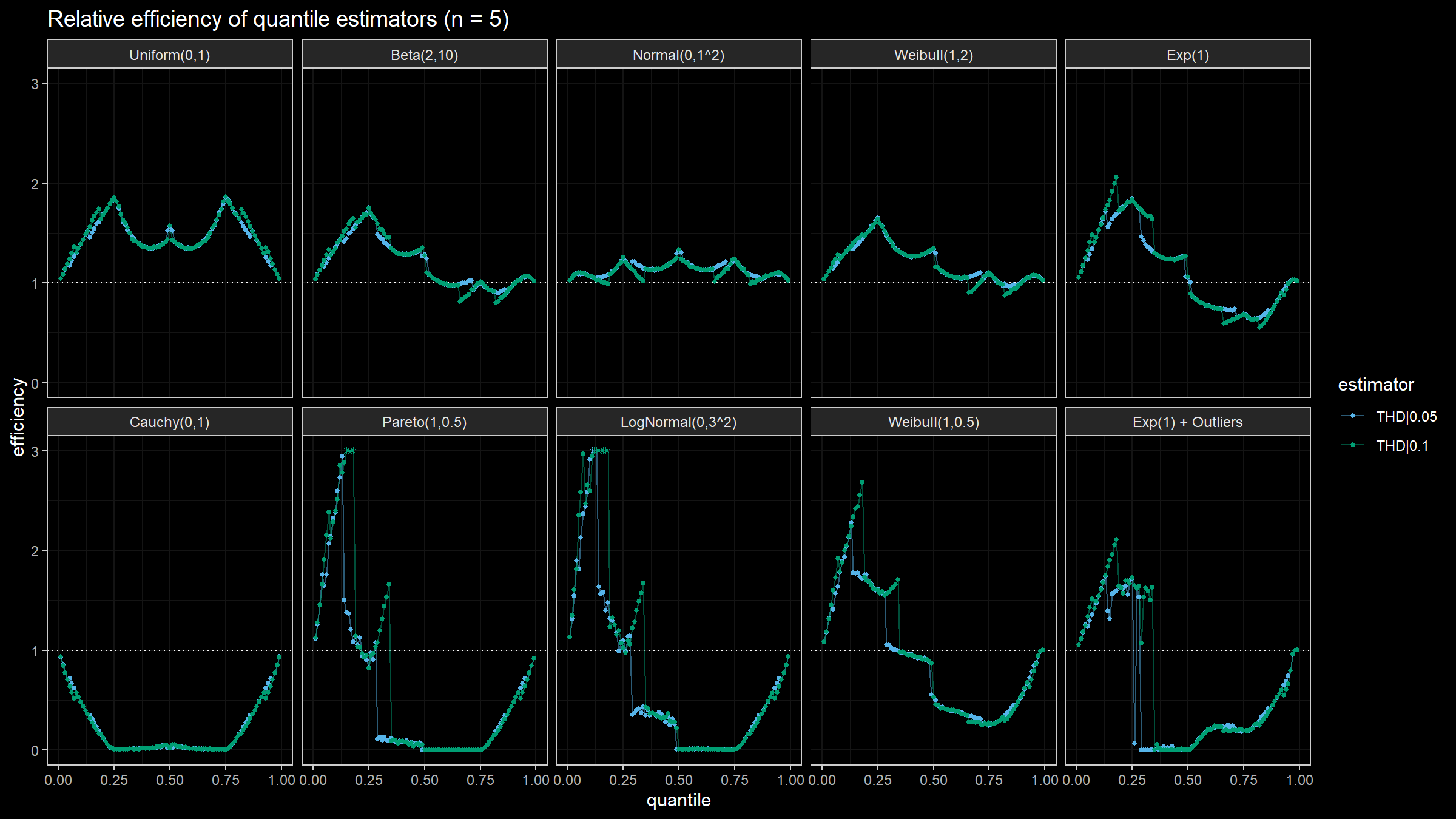
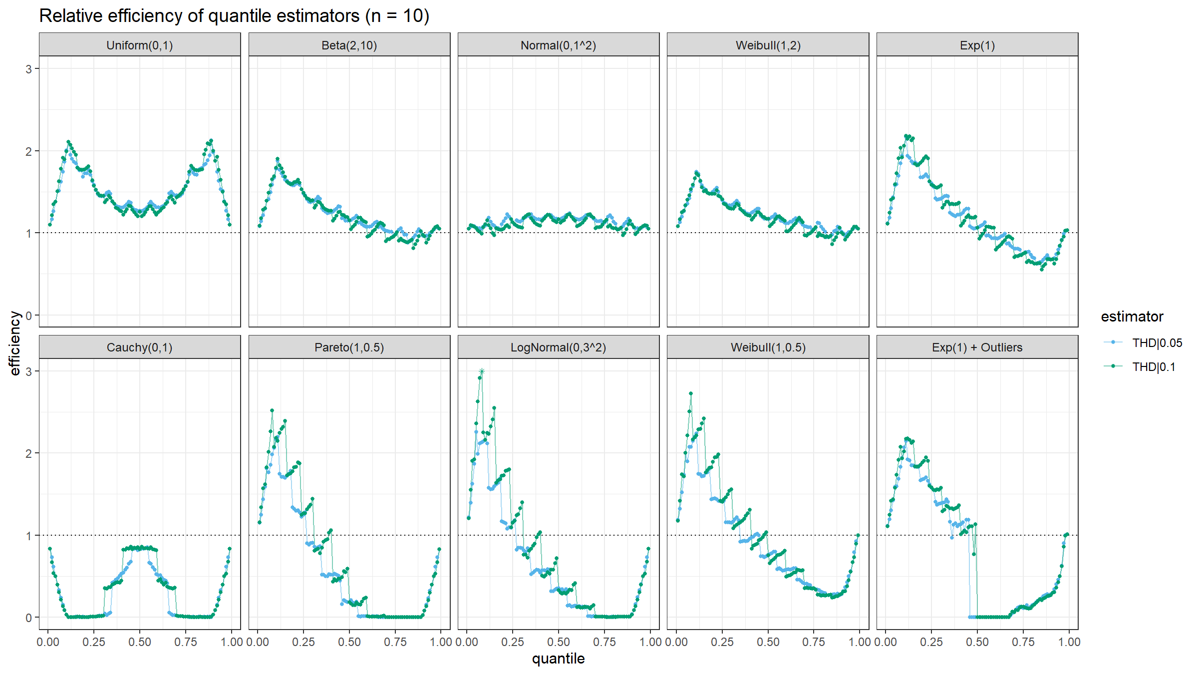
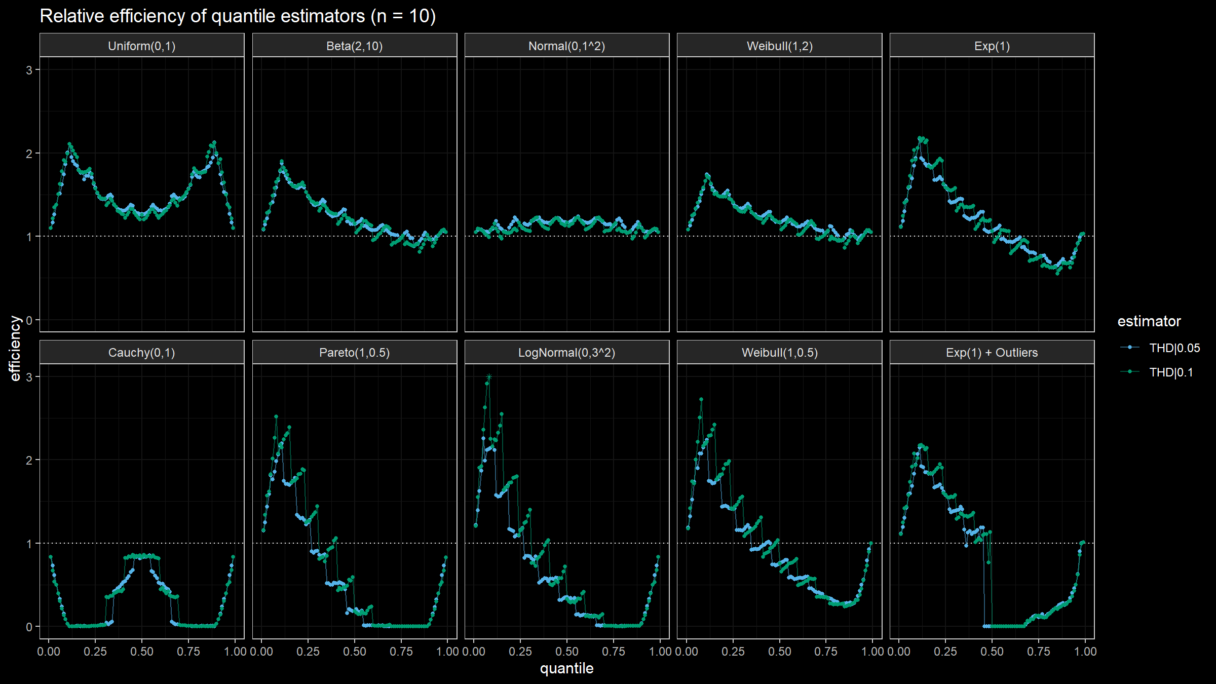
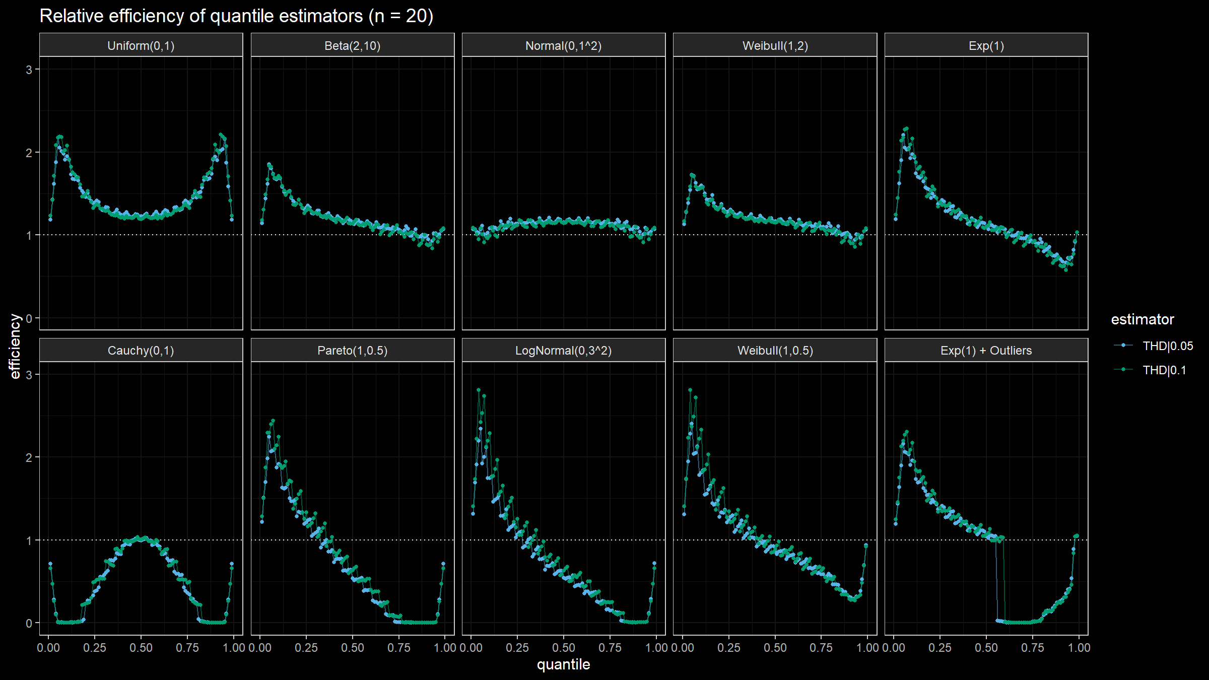
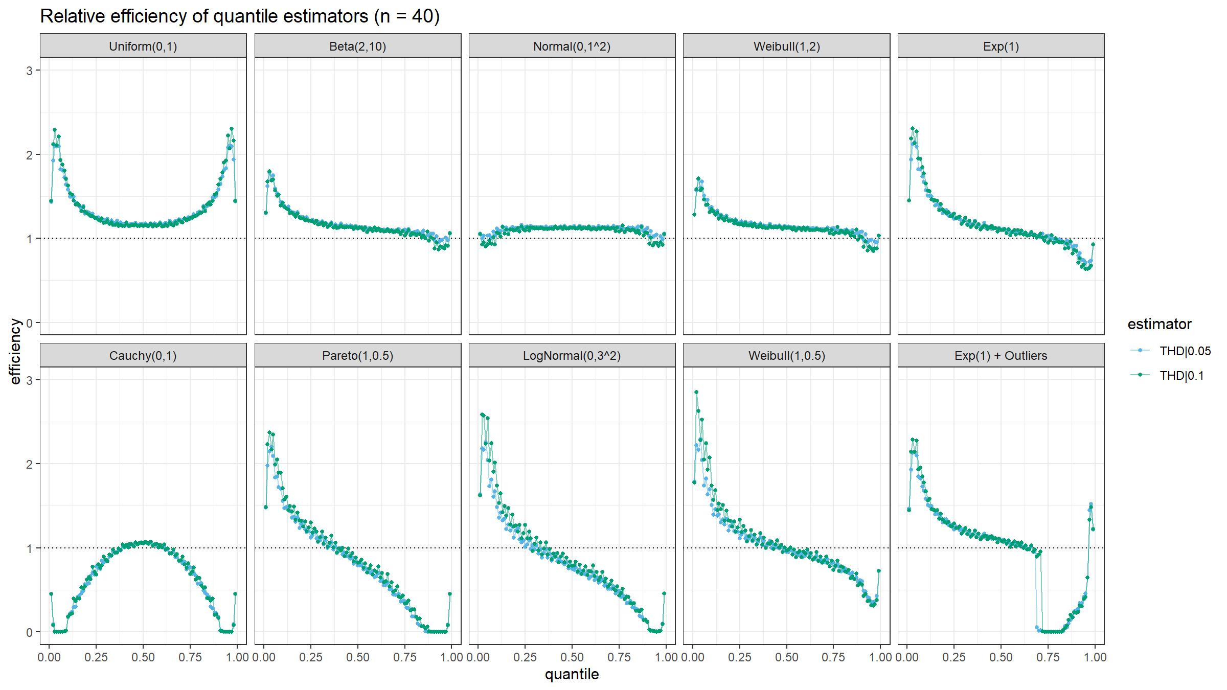
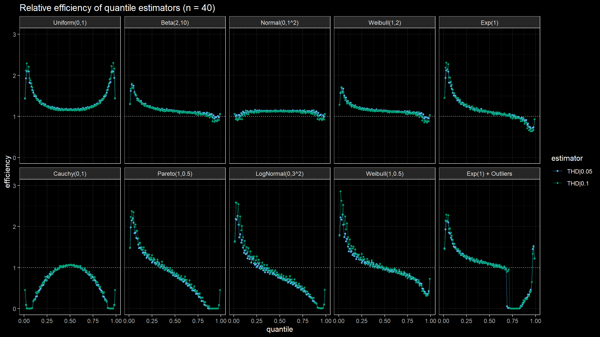
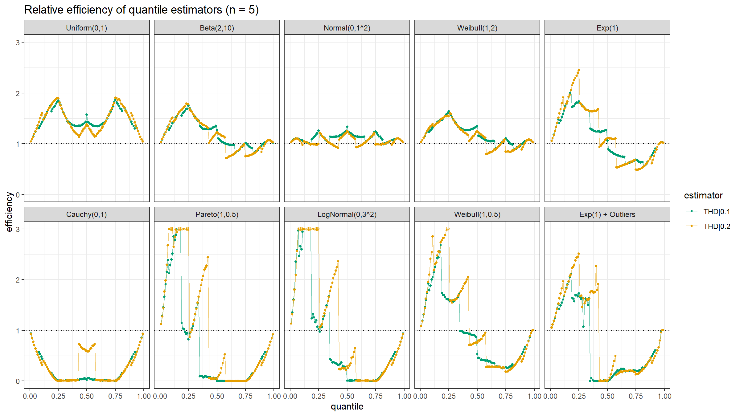
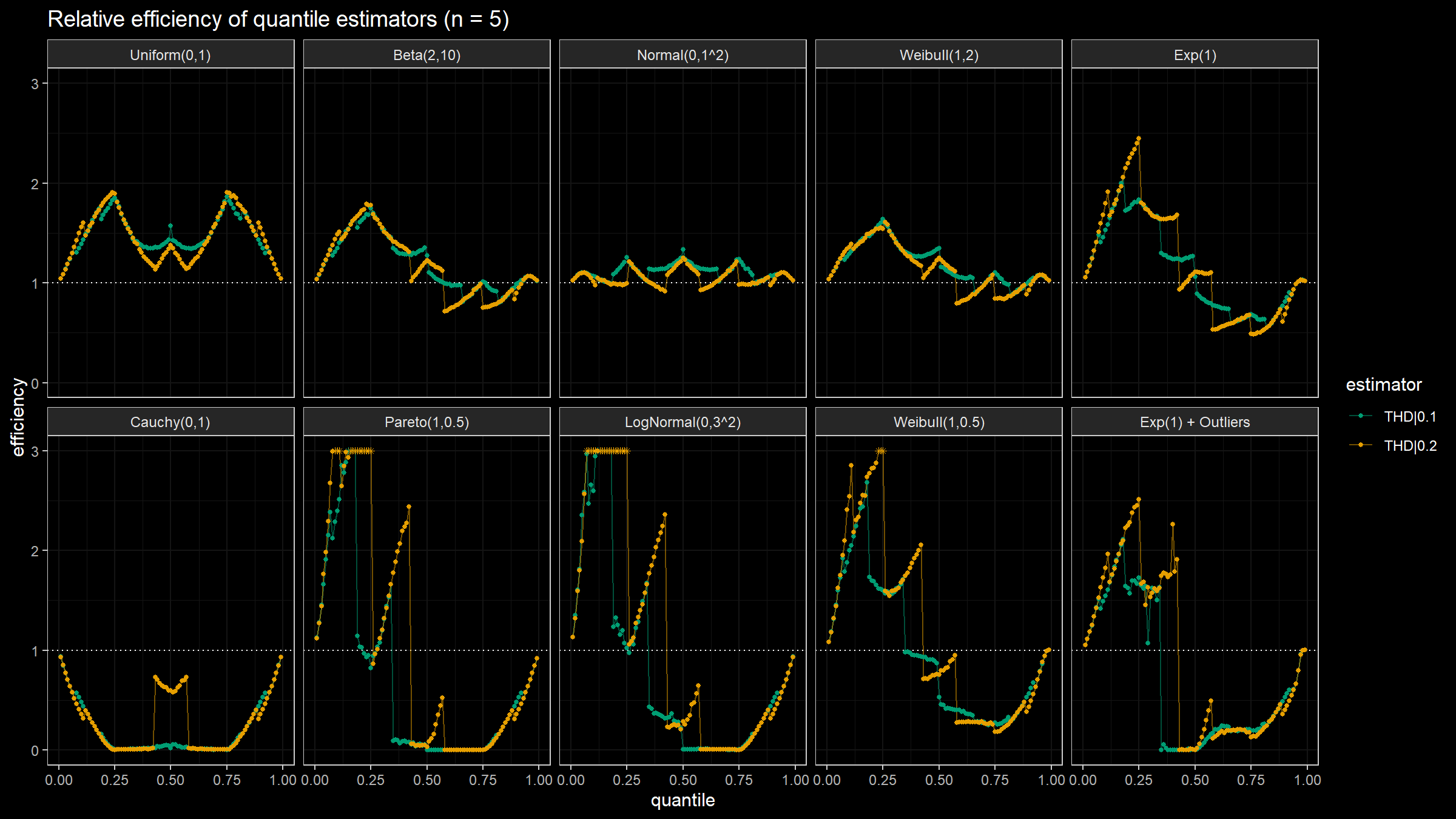
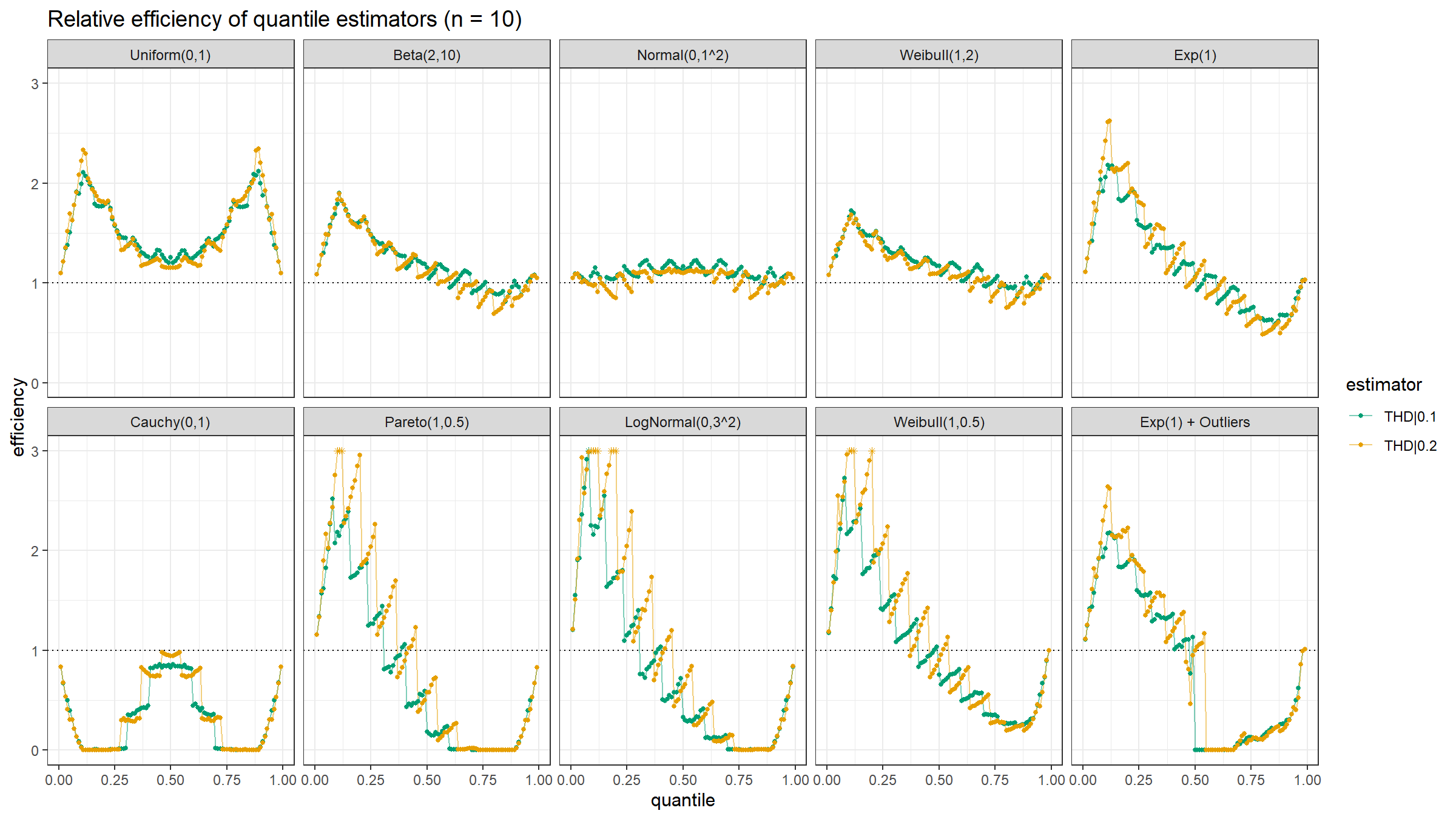
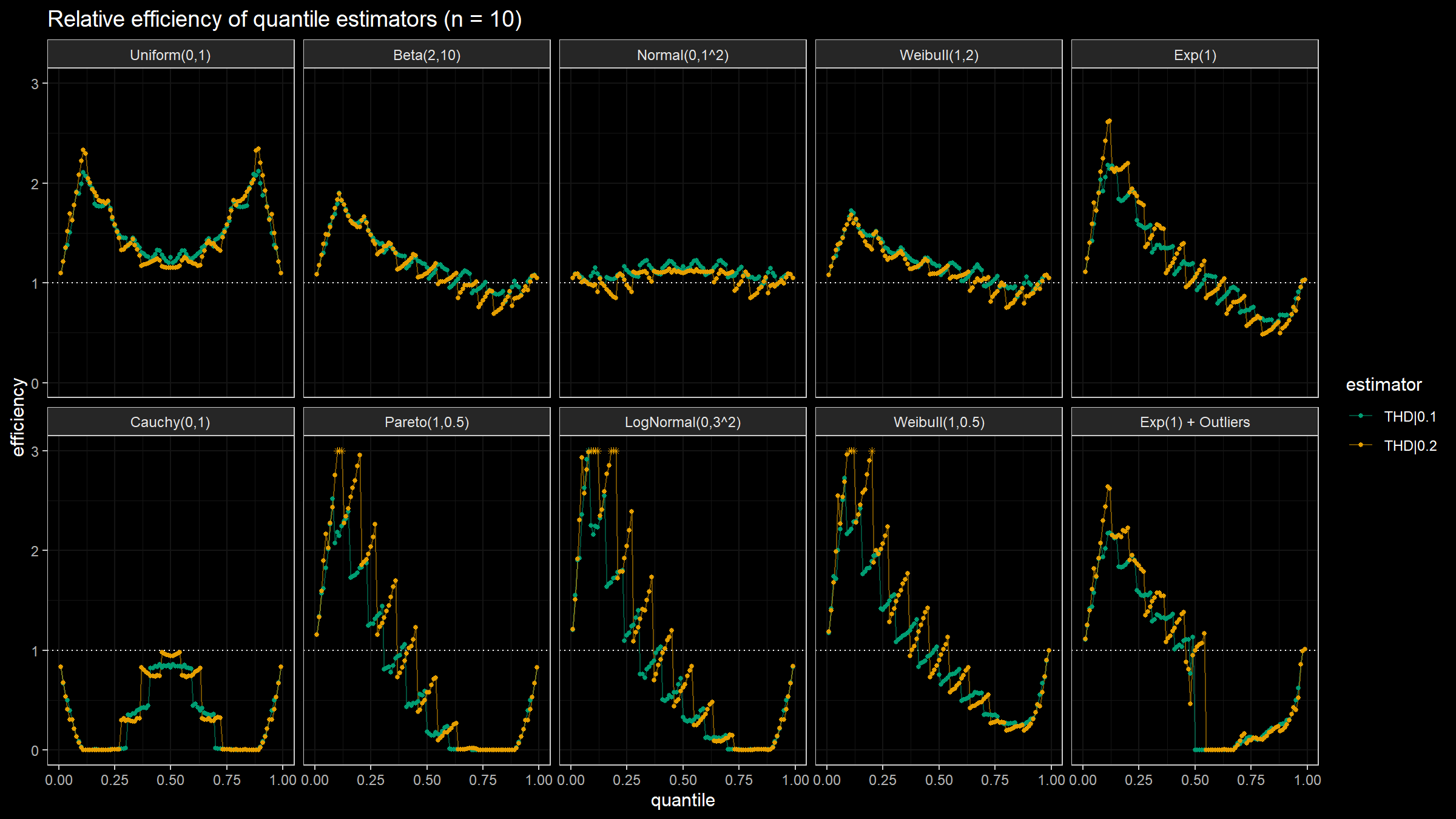
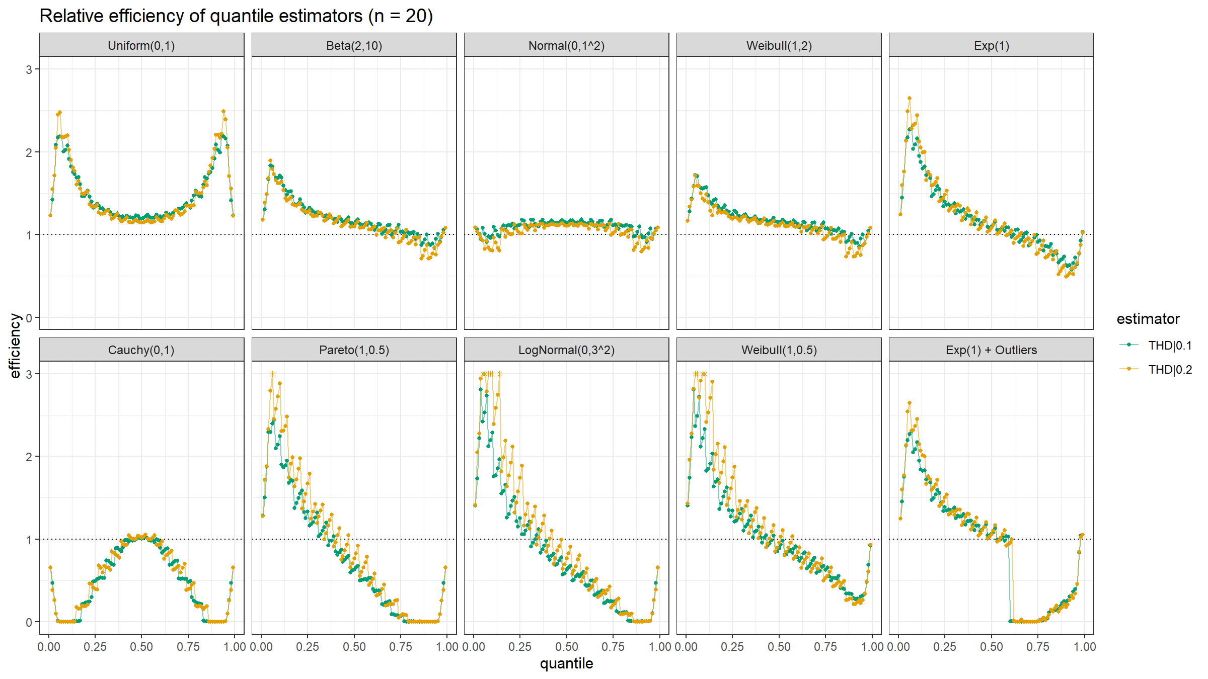
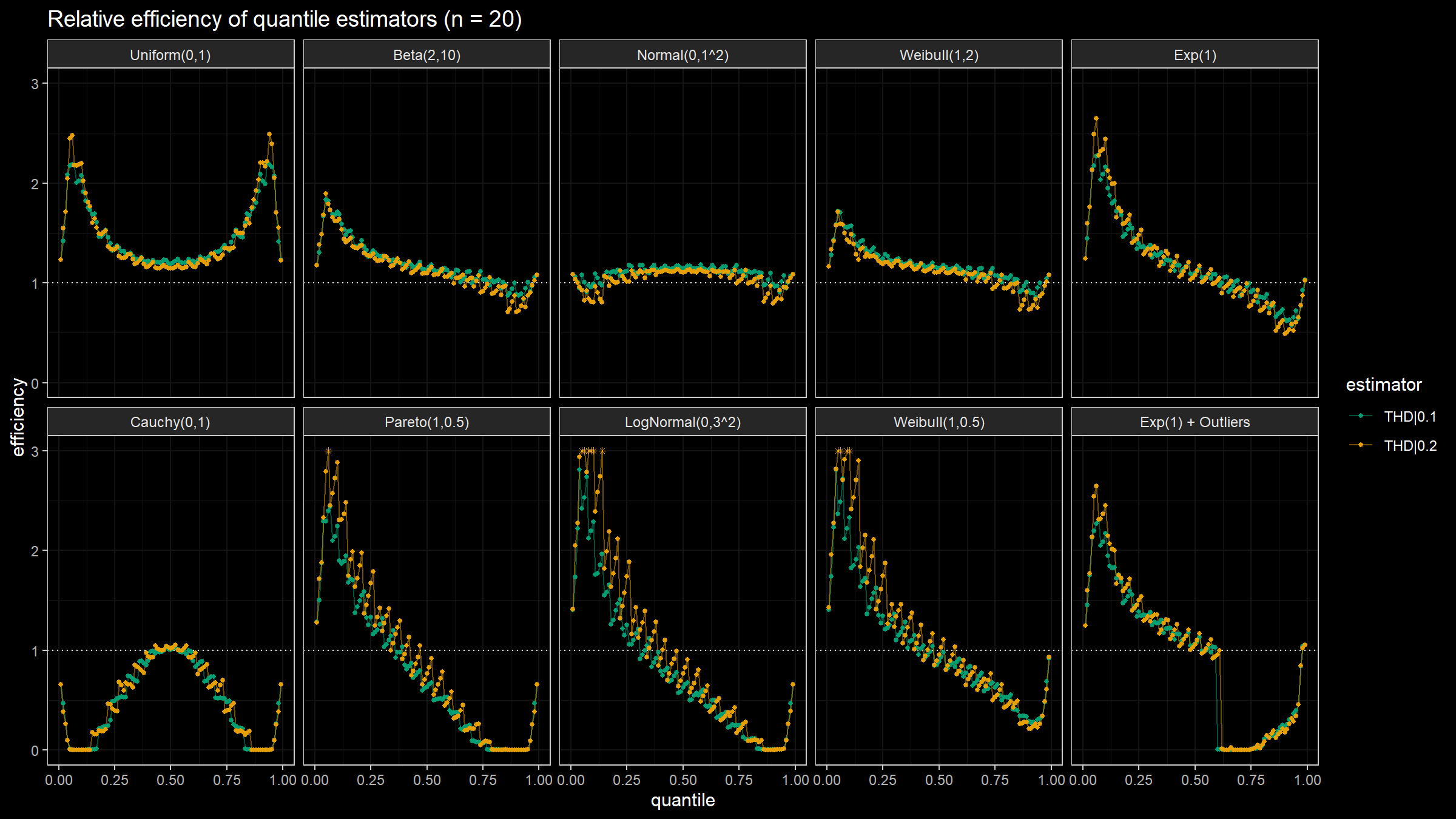
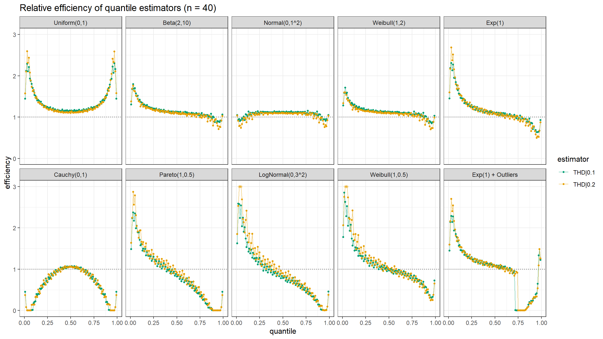
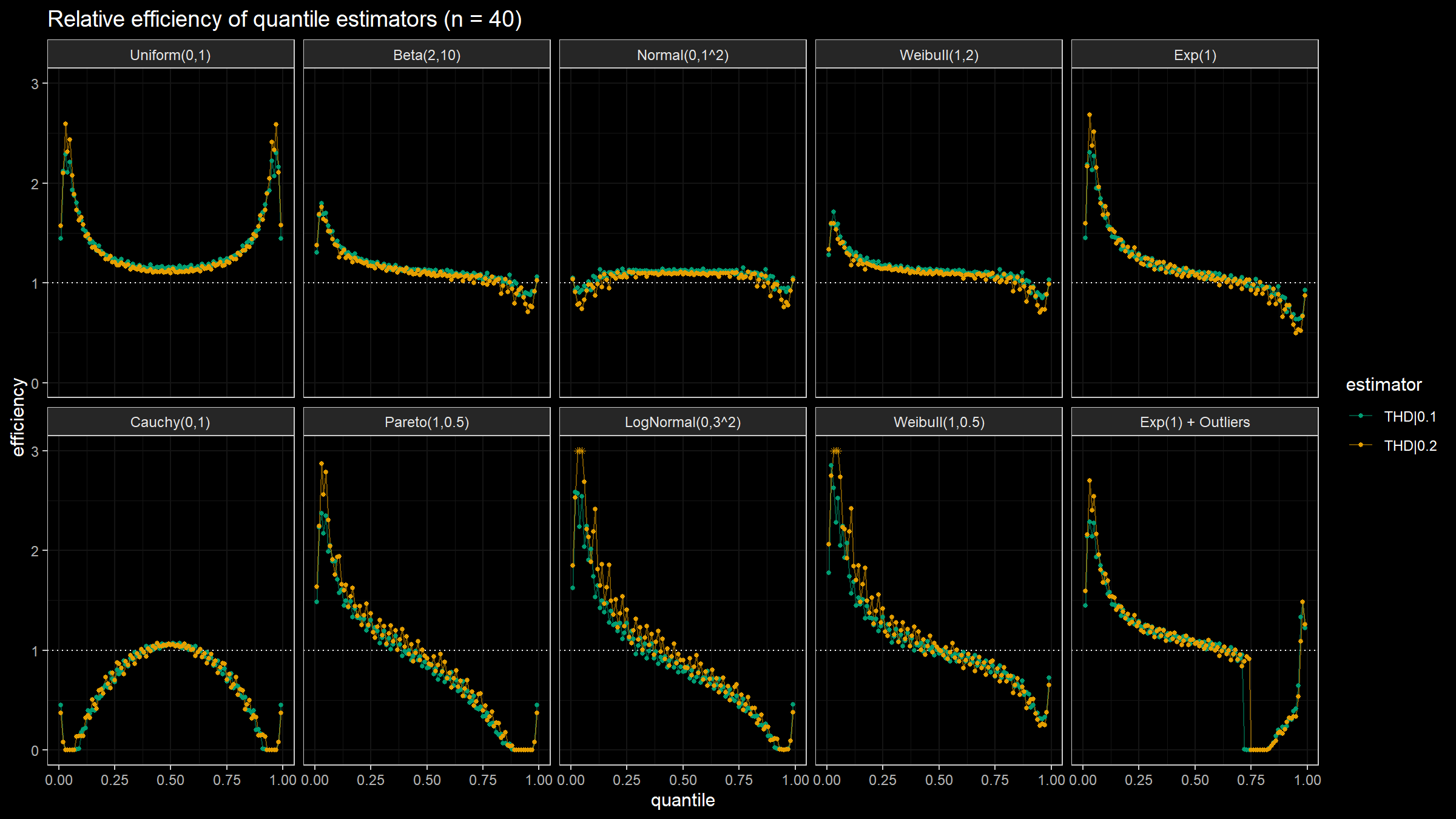
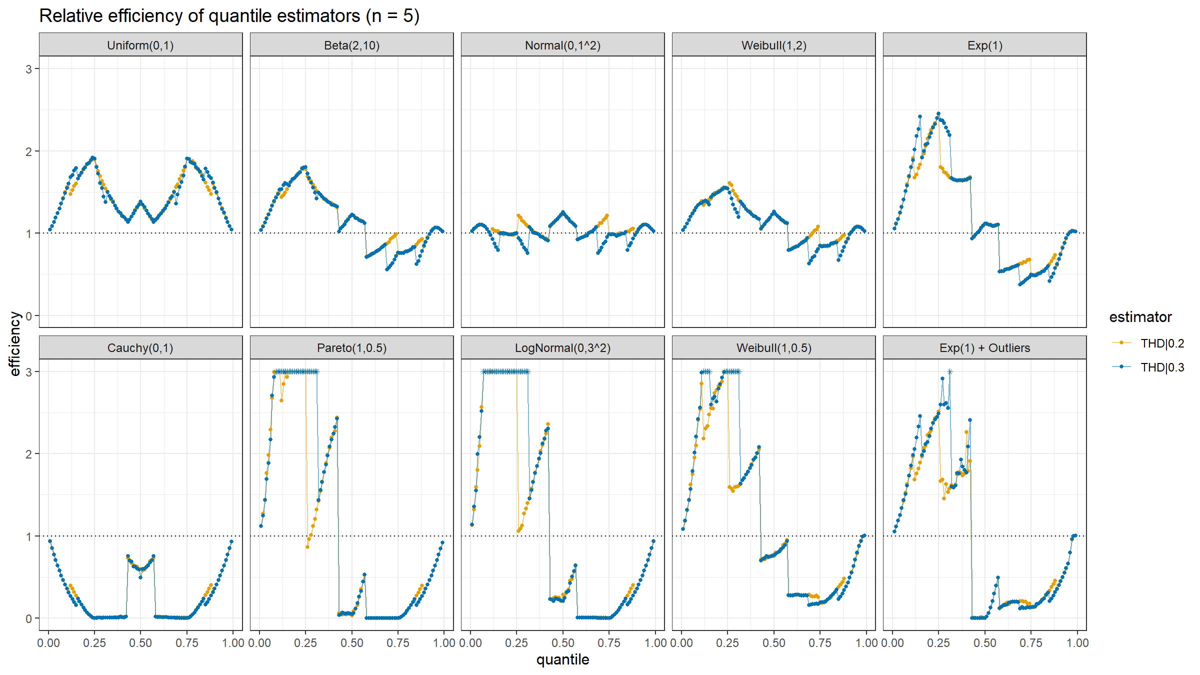
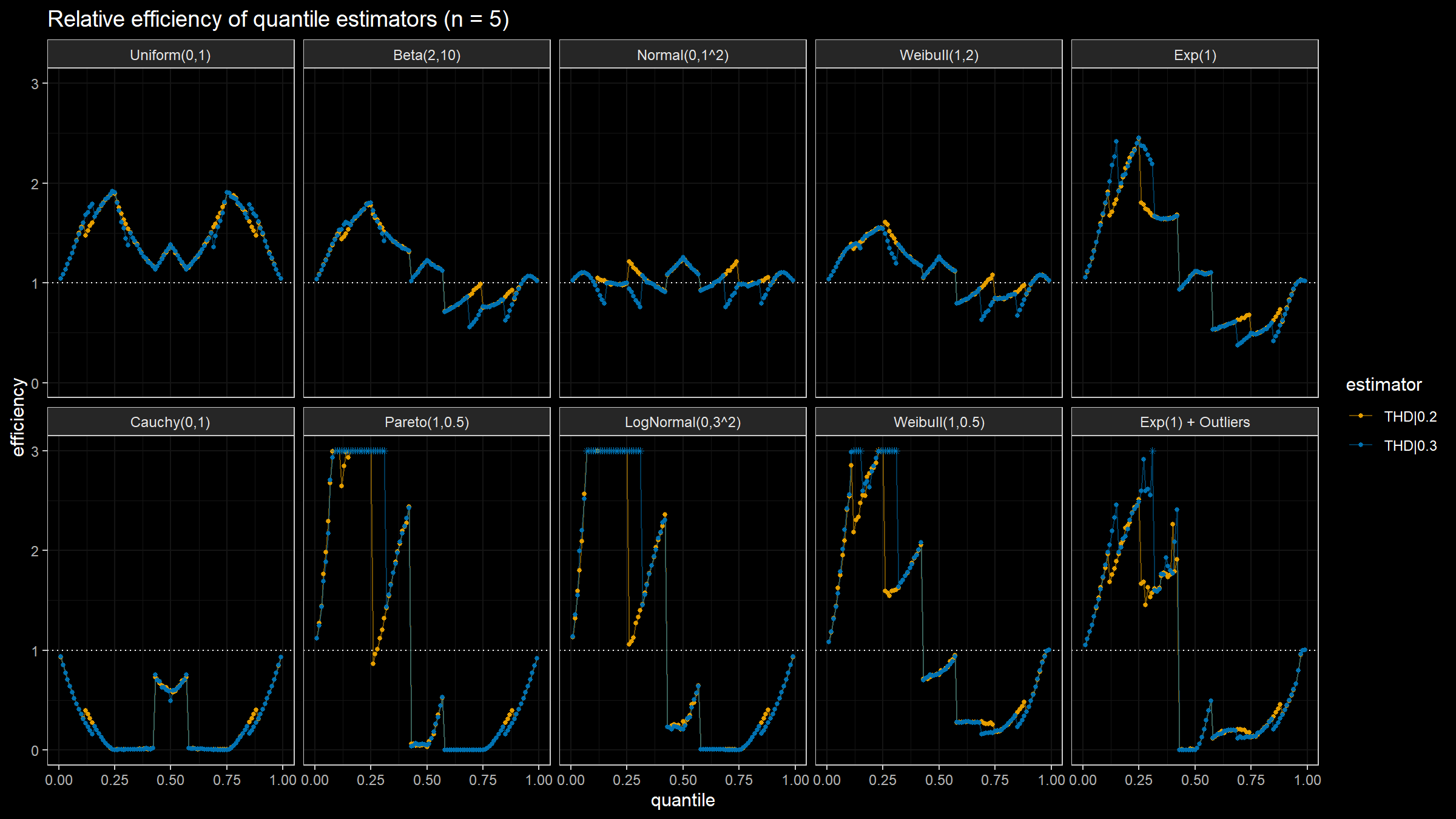
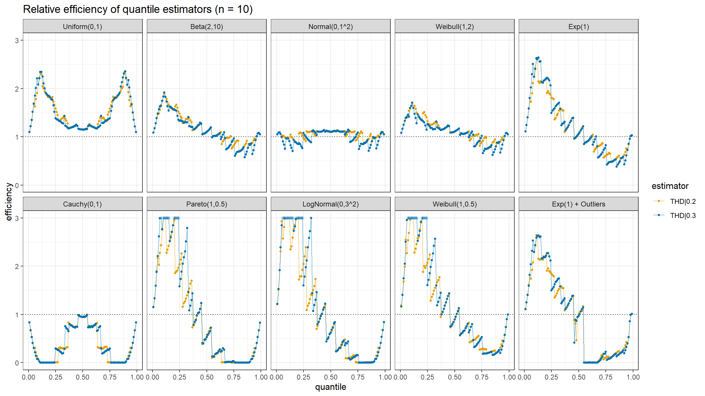
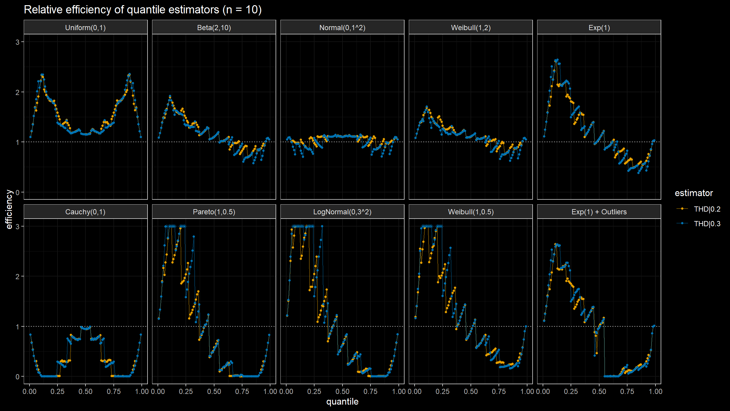
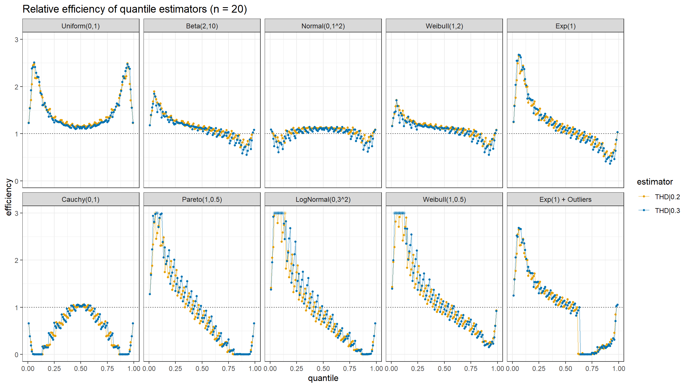
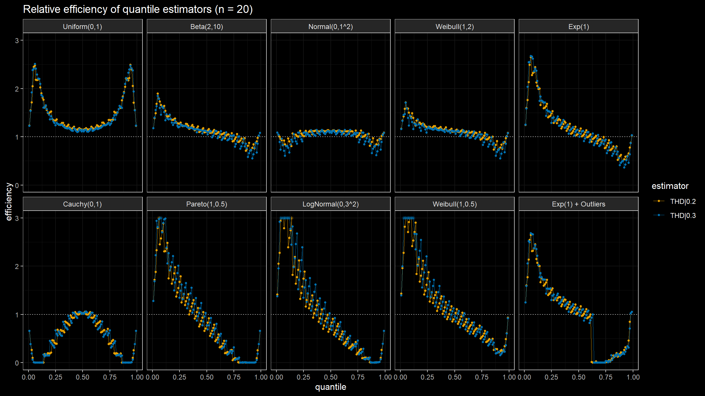
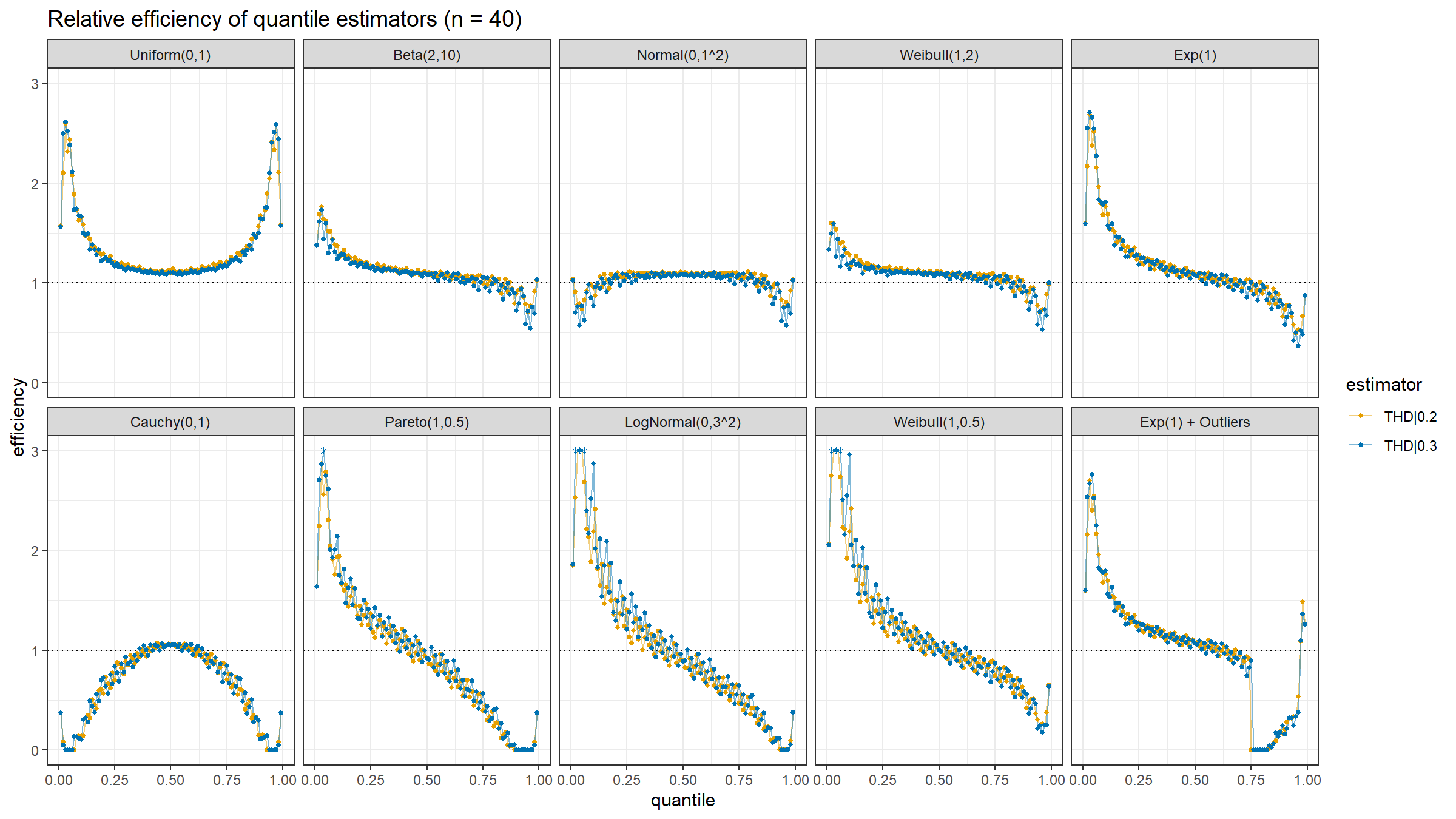
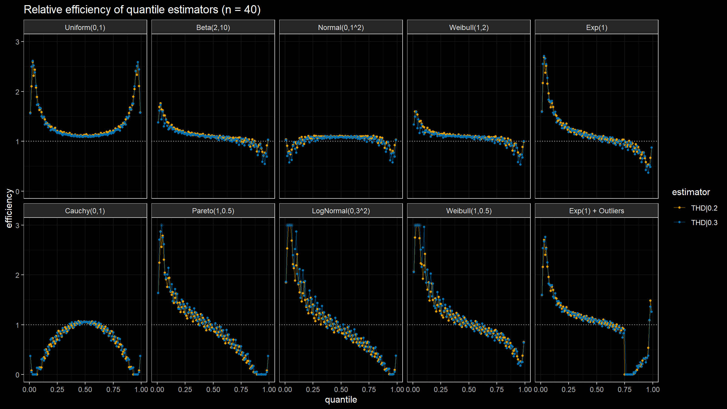
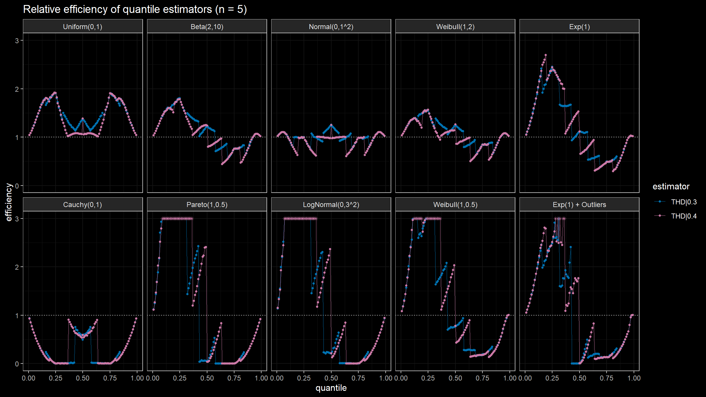
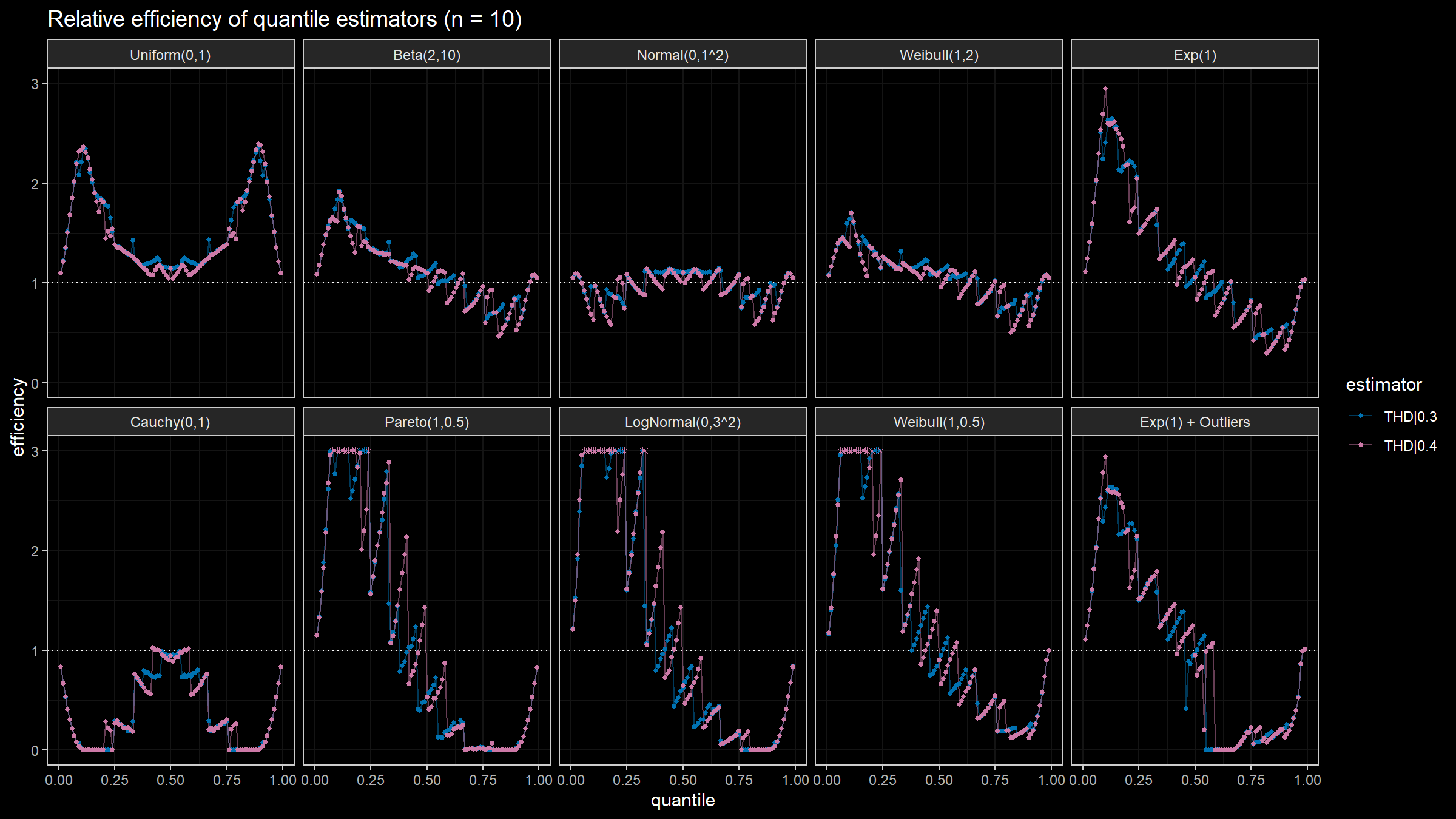
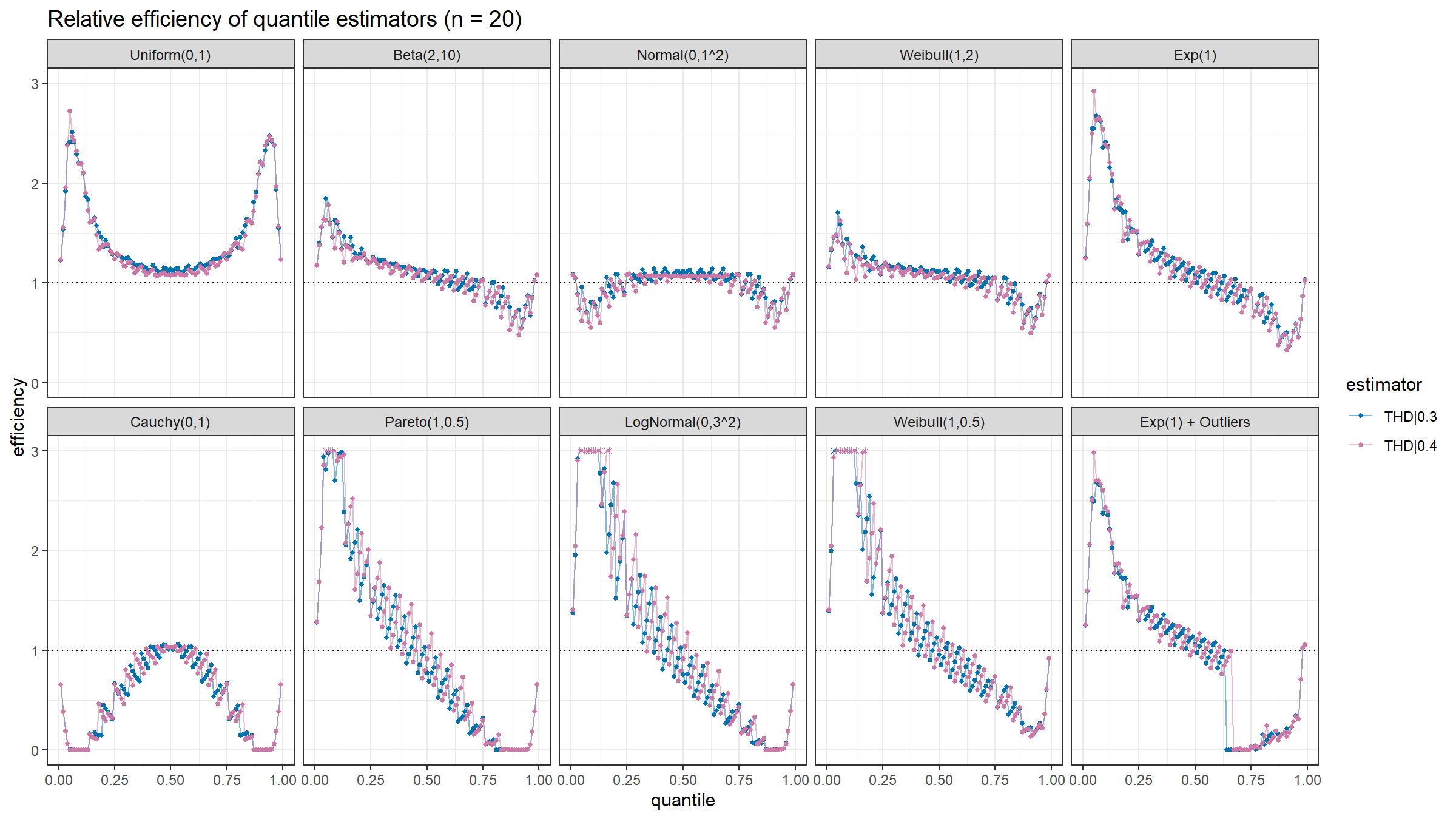
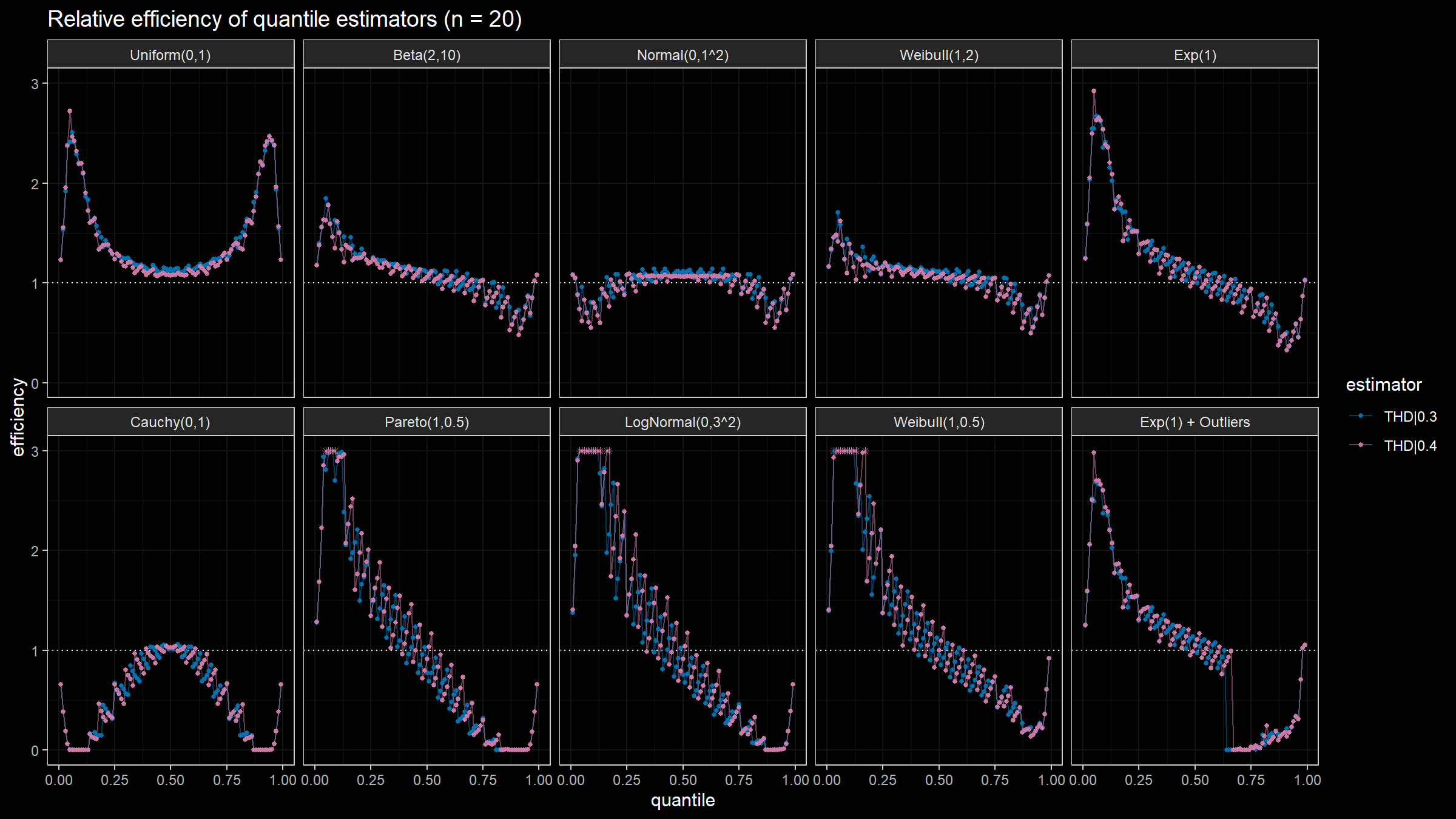
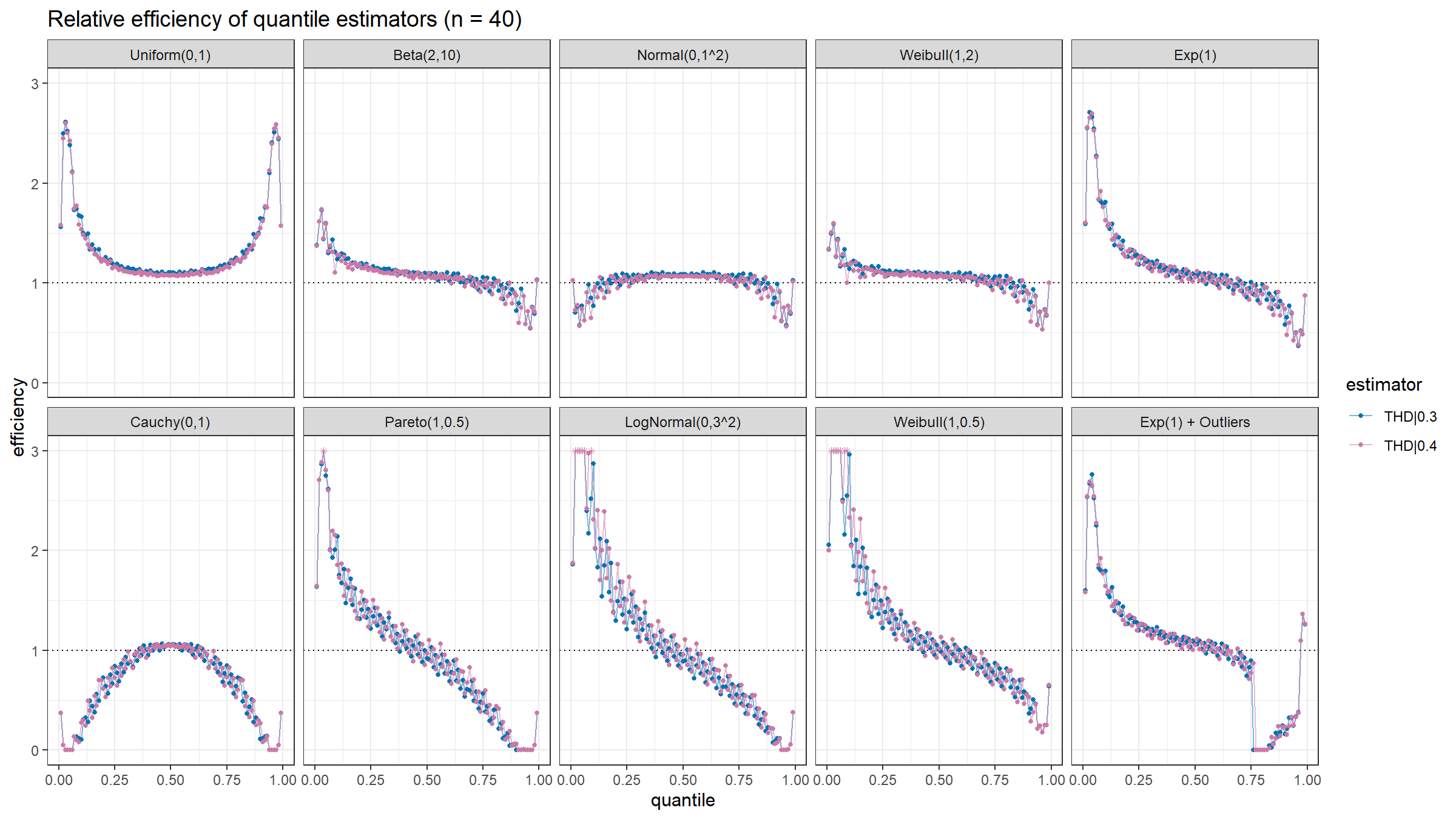
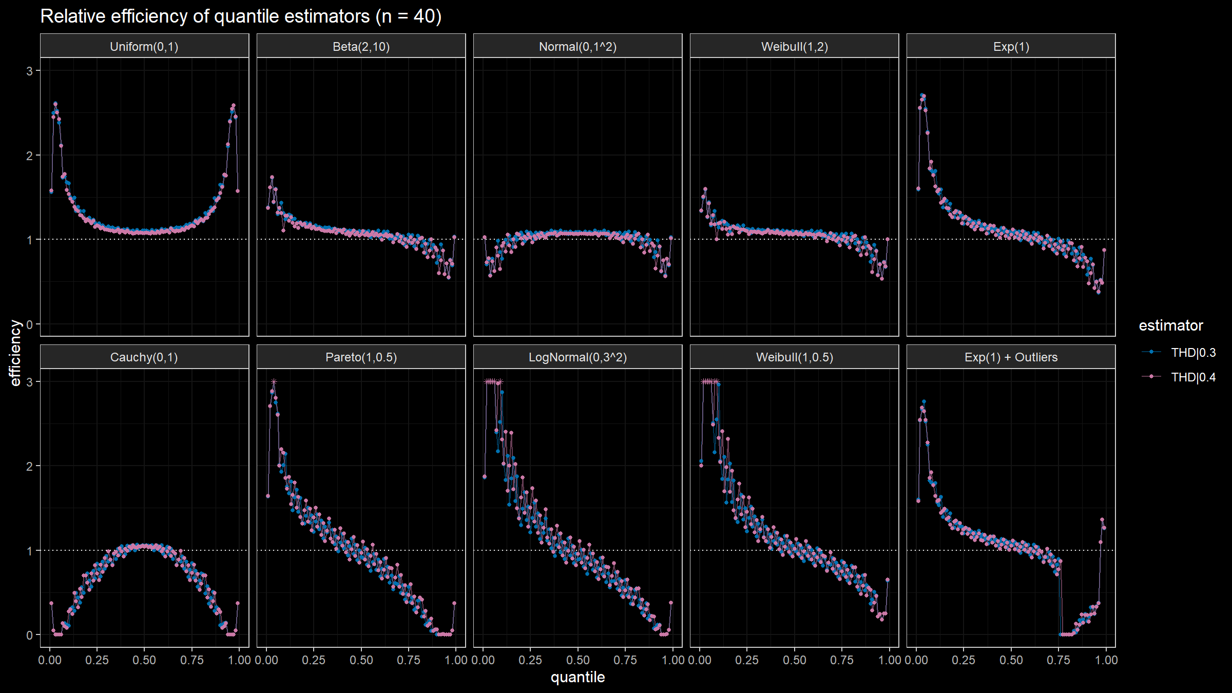
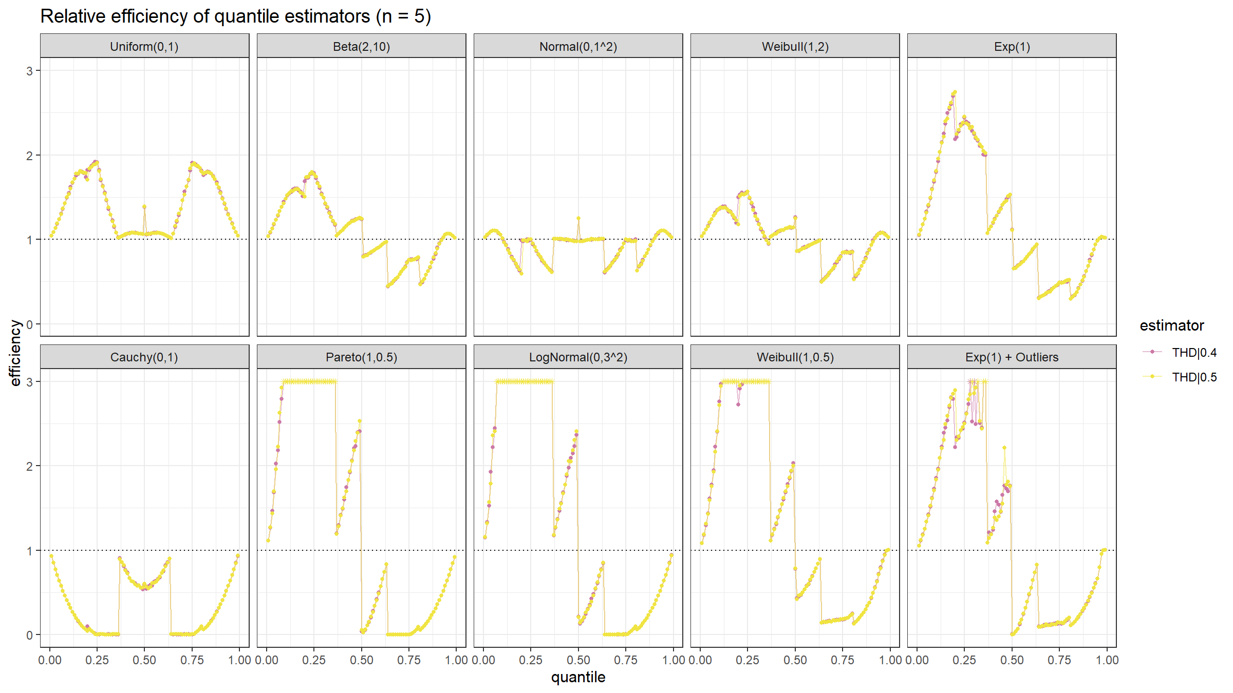
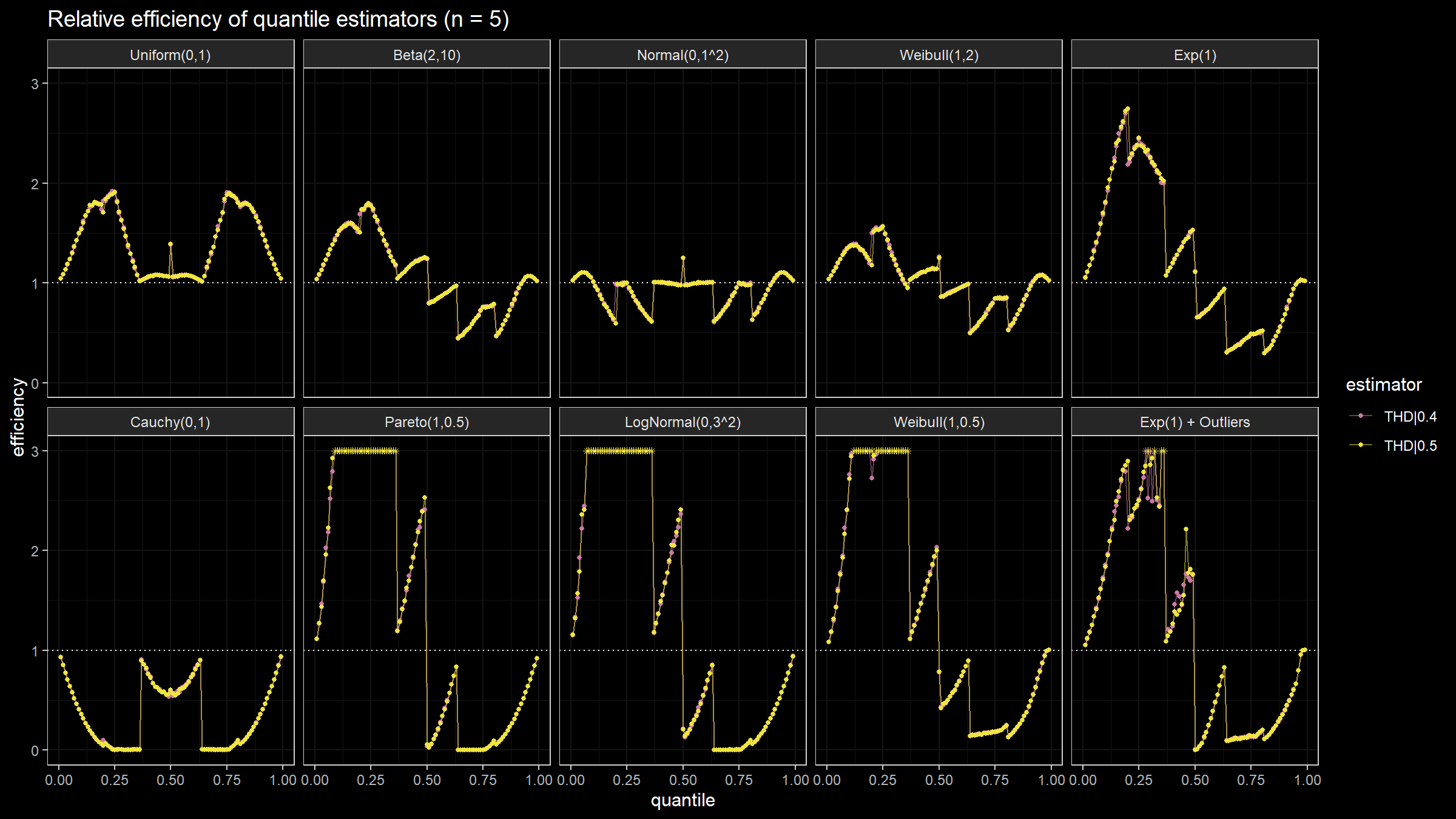
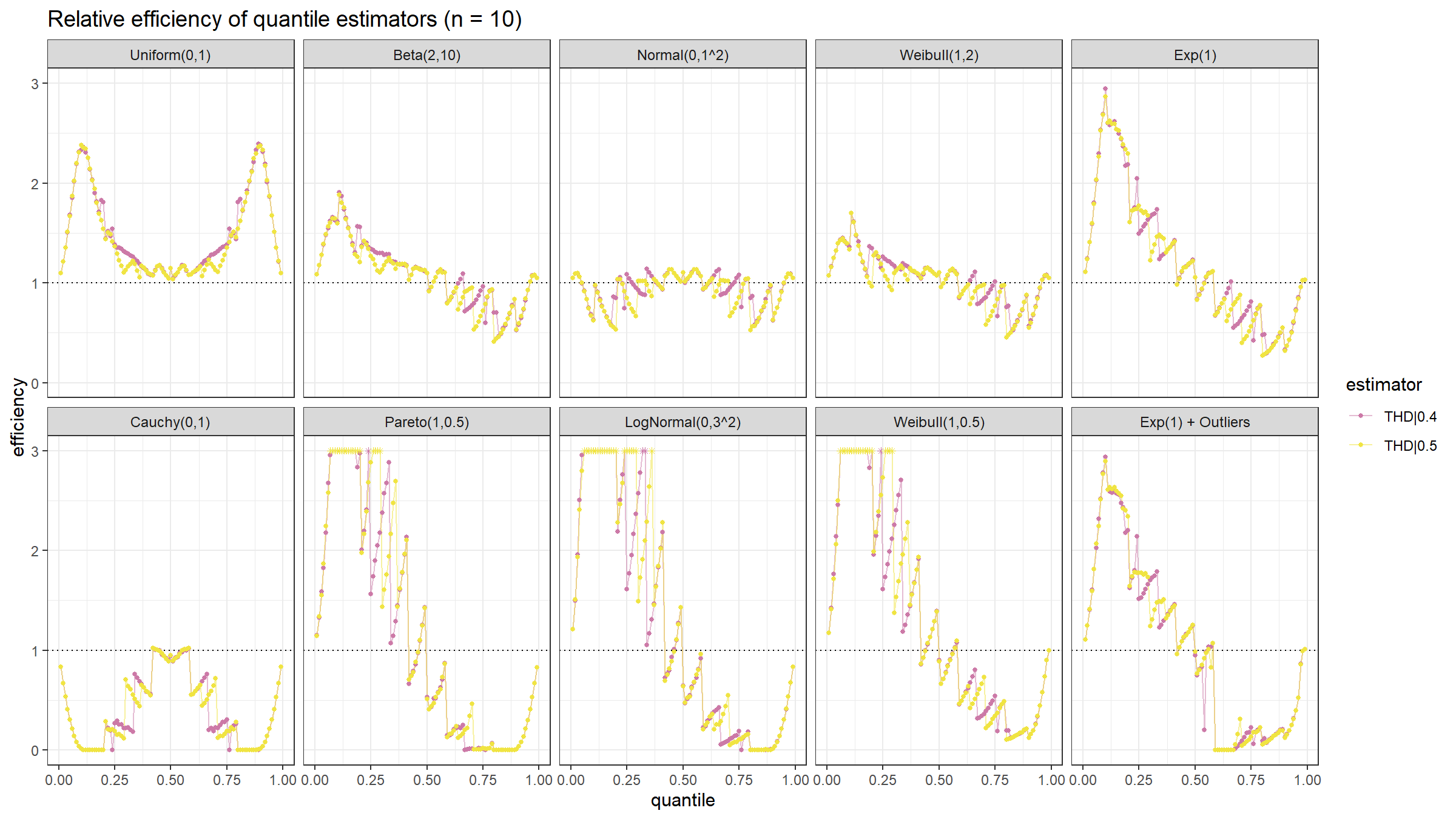
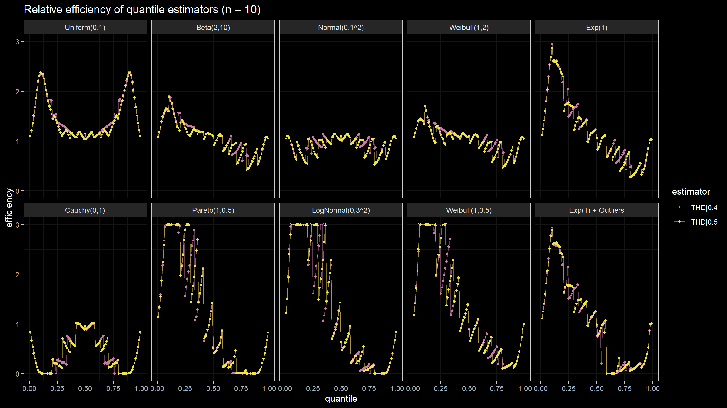
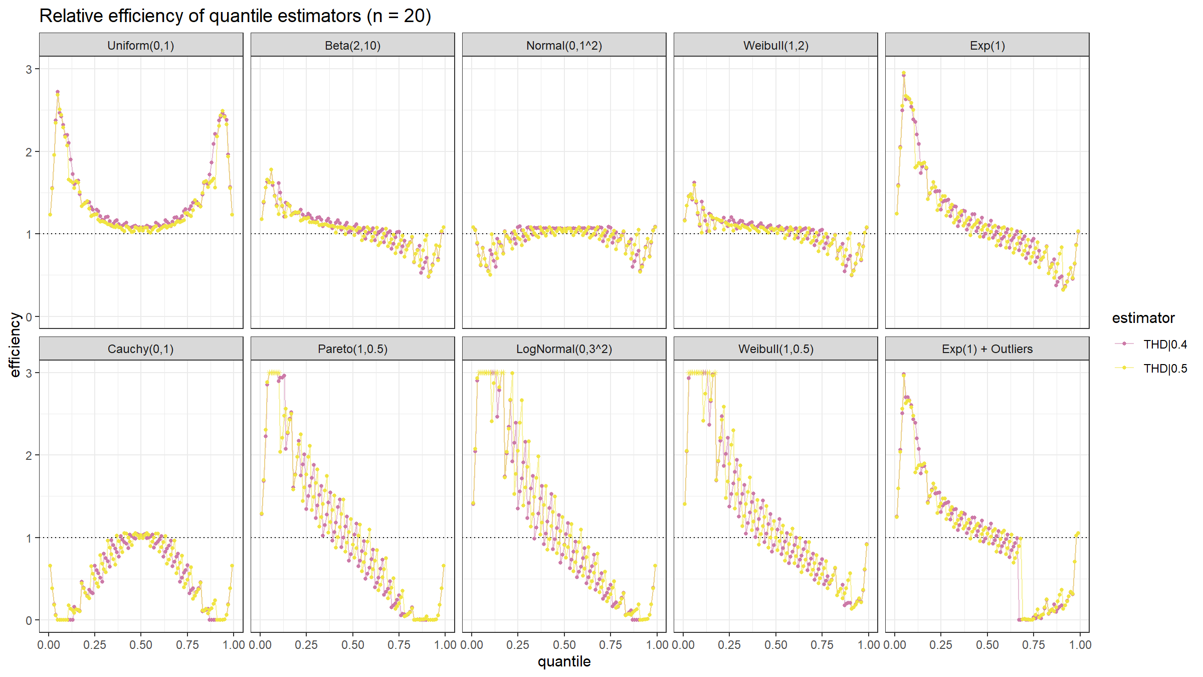
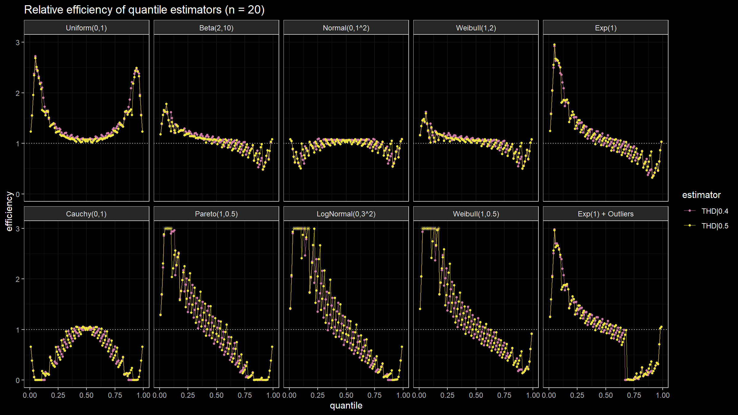
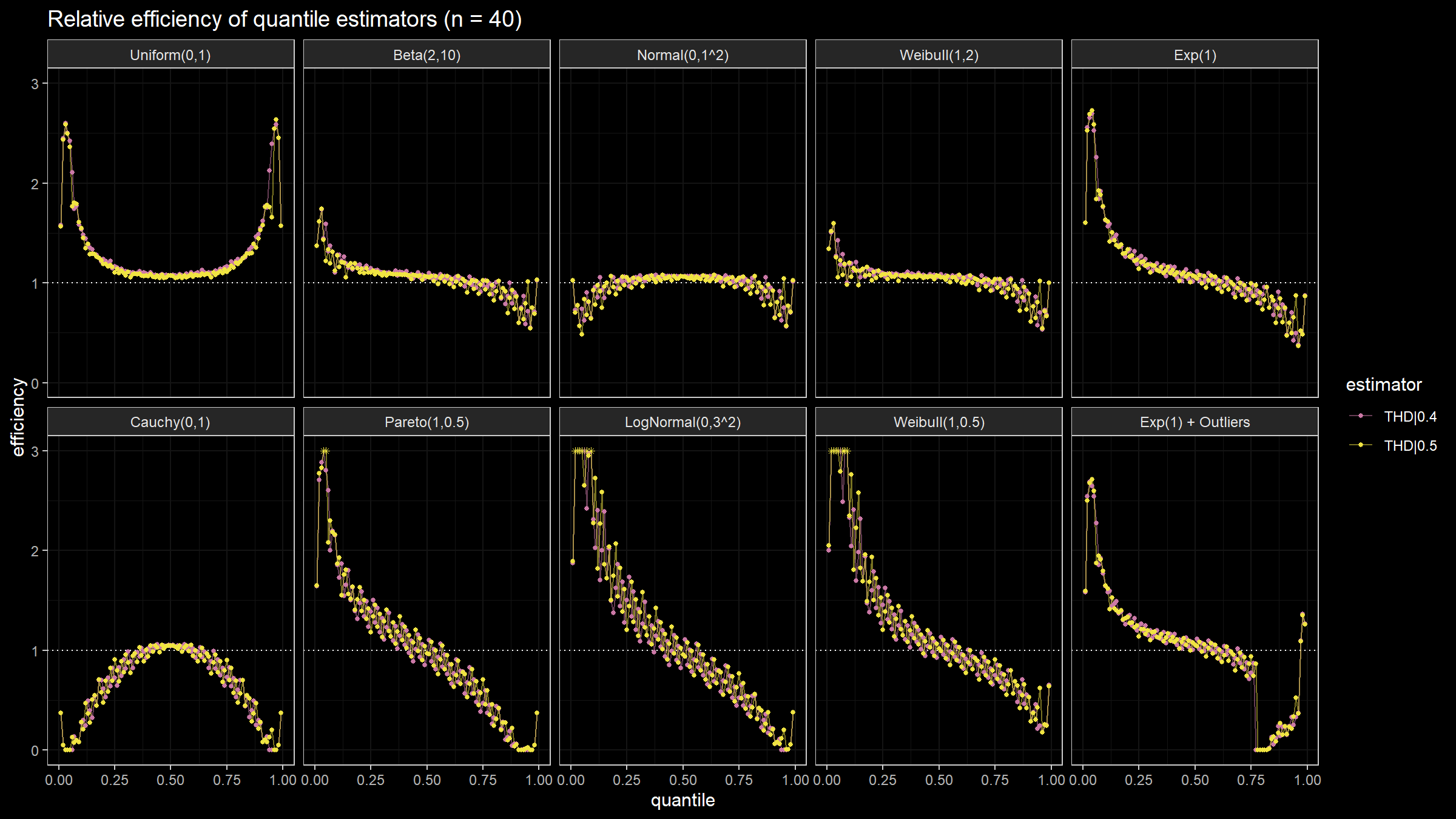
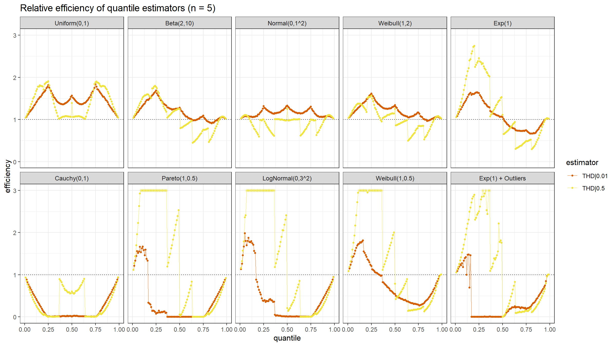
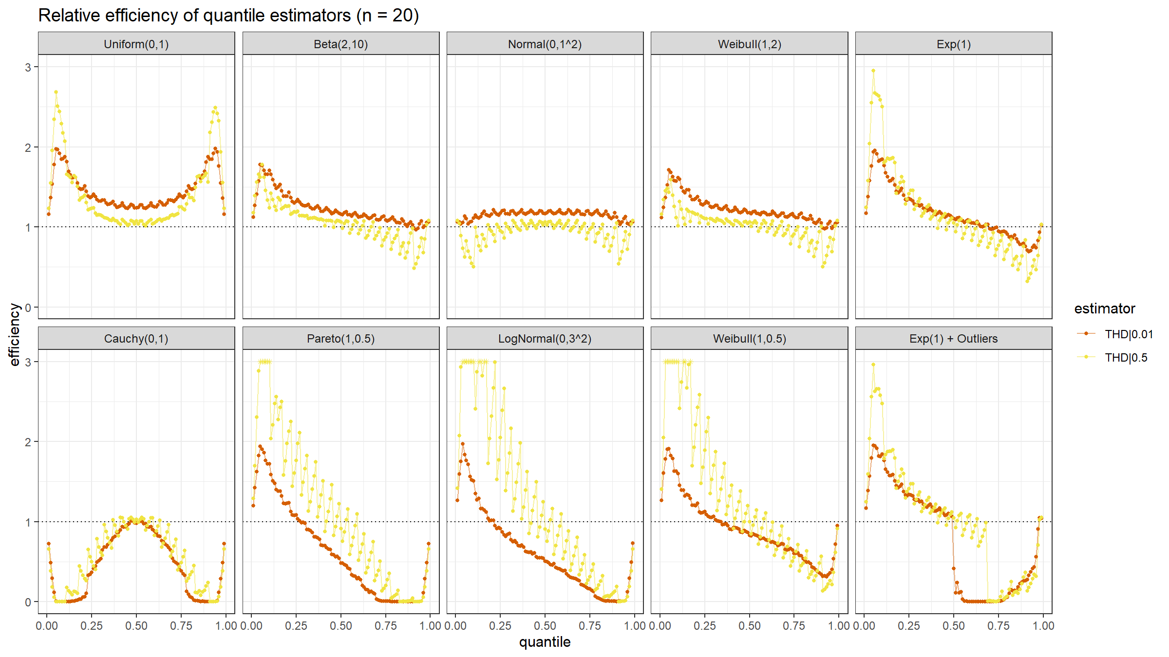
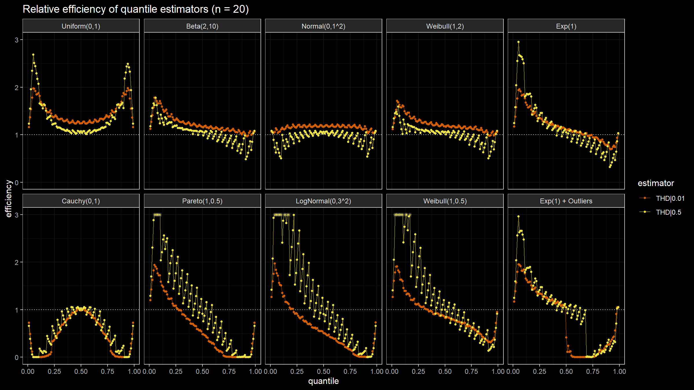
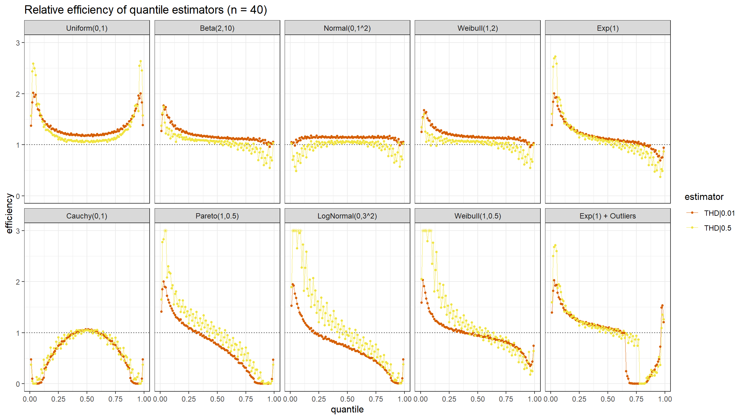
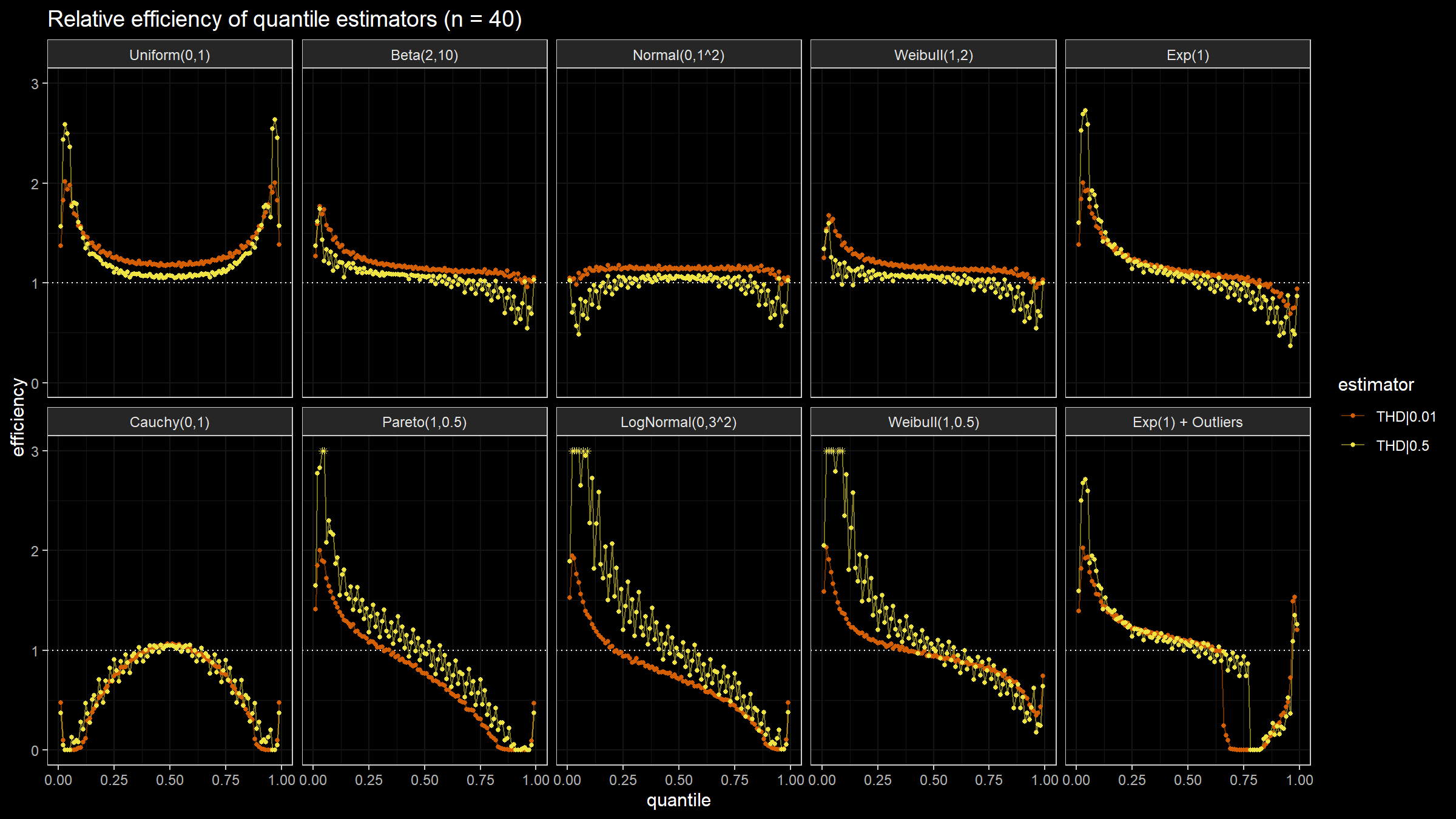
Below you can find static images for different trimming percentages and sample size values.

Conclusion

It seems there is no “optimal” threshold value. The statistical efficiency heavily depends on the underlying distributions. For light-heavy distributions, a small (or even zero) trimming percentage is preferable because it provides the highest efficiency. However, for heavy-tailed distributions, it makes sense to increase the trimming percentage value in order to improve robustness.

Based on my experience, if you expect to have some outlier values, it’s a good idea to set the trimming percentage value between 1% and 10%.

References

• [Harrell1982]
  Harrell, F.E. and Davis, C.E., 1982. A new distribution-free quantile estimator. Biometrika, 69(3), pp.635-640.
  https://doi.org/10.2307/2335999
• [Hyndman1996]
  Hyndman, R. J. and Fan, Y. 1996. Sample quantiles in statistical packages, American Statistician 50, 361–365.
  https://doi.org/10.2307/2684934