Trimmed modification of the Harrell-Davis quantile estimator

In one of the previous posts, I discussed winsorized Harrell-Davis quantile estimator. This estimator is more robust than the classic Harrell-Davis quantile estimator. In this post, I want to suggest another modification that may be better for some corner cases: the trimmed Harrell-Davis quantile estimator.

Winsorizing

I already discussed winsorization of the Harrell-Davis quantile estimator in detail in my previous post. Let’s briefly recall the main idea. For sample $x = \{ x_1, x_2, \ldots, x_n \}$, the Harrell-Davis quantile estimator (harrell1982) estimates the $p^\textrm{th}$ quantile using the following equation:

$$ Q_{HD}(p) = \sum_{i=1}^{n} W_{i} \cdot x_{(i)}, \quad W_{i} = I_{i/n}(a, b) - I_{(i-1)/n}(a, b), \quad a = p(n+1),\; b = (1-p)(n+1) $$

where $I_t(a, b)$ denotes the regularized incomplete beta function, $x_{(i)}$ is the $i^\textrm{th}$ order statistic.

This approach is quite effective (you can find relevant simulations here). Unfortunately, it’s not robust because it’s a sum of all order statistics with positive weights. The breakdown point of such a metric is zero: a single outlier may corrupt the estimation of any quantile.

Now let’s look at an example. Here is the probability density function plot of the beta distribution for $n = 20, p = 0.2$:

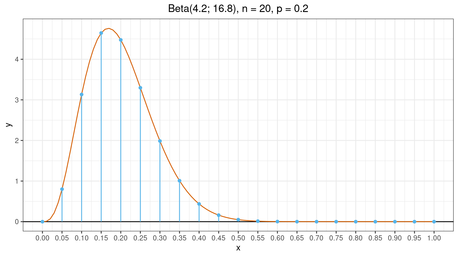
Blue vertical lines split the plot into 20 fragments. The value of $W_i$ is the area of $i^\textrm{th}$ fragment. As you can see, half of the fragments have tiny areas which are close to zero. Meanwhile, these fragments are also the reason of the zero breakdown point. Thus, we have the following situation:

• If there are no extreme values, tiny fragments don’t produce a noticeable contribution to the estimation value.
• If there are extreme values, tiny fragments may corrupt the estimation value because their areas are actually positive.

Therefore, such tiny fragments don’t improve efficiency and reduce robustness. Moreover, they noticeably slow down numerical calculation because it takes some time to evaluate all values of the regularized incomplete beta function. So, what’s the point of including such fragments in the calculations? Let’s get rid of them! We can consider two strategies of eliminating tiny fragments.

The first strategy is winsorization which I suggested in the previous posts. The idea is pretty simple. Let’s find the k% highest density interval (e.g., we can consider k=95 or k=99). Next, we find all the fragments that overlap with this interval. Let’s say such fragments have indexes from $l$ to $r$. The winsorization assumes that we replace all values between $1$ and $l-1$ by $x_{(l)}$ and replace all values between $r+1$ and $n$ by $x_{(r)}$. Here is the final equation for the winsorized Harrell-Davis (WHD) quantile estimator:

$$ Q_{WHD}(p) = \sum_{i=1}^{l-1} W_i \cdot x_{(l)} + \sum_{i=l}^{r} W_i \cdot x_{(i)} + \sum_{i=r+1}^{n} W_i \cdot x_{(r)}. $$

Thus, if we have outliers outside the $[l..r]$ interval, they won’t corrupt the quantile estimation. The same trick could be applied to the Maritz-Jarrett method ([Maritz1979]) to estimate corresponding winsorized quantile confidence interval.

Trimming

Trimming is very similar to winsorizing with two differences:

• Instead of replacing $x_{(i)}$ outside the $[l..r]$ interval, we should eliminate them.
• Since the sum of all weights should be equal to one, we should normalize $W_i$ values.

Here is the final equation for the trimmed Harrell-Davis (THD) quantile estimator:

$$ Q_{THD}(p) = \dfrac{1}{\sum_{i=l}^{r} W_i} \sum_{i=l}^{r} W_i \cdot x_{(i)}. $$

In most cases, winsorized and trimmed modifications provide similar results. We can observe a noticeable difference between them when $x_{(l)}$ or $x_{(r)}$ is an outlier. In this case, the trimmed modification seems to be more efficient because it assigns lower weight to the extreme value. I’m going to share some numerical experiments related to the efficiency of both modifications in our of my future blog posts.

Reference implementation

The C# reference implementation can be found in the latest nightly version (0.3.0-nightly.92+) of Perfolizer (you need TrimmedHarrellDavisQuantileEstimator).

References

• [Harrell1982]
  Harrell, F.E. and Davis, C.E., 1982. A new distribution-free quantile estimator. Biometrika, 69(3), pp.635-640.
  https://doi.org/10.2307/2335999
• [Maritz1979]
  Maritz, J. S., and R. G. Jarrett. 1978. “A Note on Estimating the Variance of the Sample Median.” Journal of the American Statistical Association 73 (361): 194–196.
  https://doi.org/10.1080/01621459.1978.10480027