Two-pass change point detection for temporary interval condensation
When we choose a change point detection algorithm, the most important thing is to clearly understand why we want to detect the change points. The knowledge of the final business goals is essential. In this post, I show a simple example of how a business requirement can be translated into algorithm adjustments.
The problem
Let us describe the context of a specific problem. We monitor the values of the performance metrics of an application. The source of these measurements does not matter: it can be server monitoring data or benchmark output from CI runs. The underlying data often do not follow known distributions, and, therefore, we should use nonparametric statistics. We want to be alerted in case of significant performance degradation. We also want to have a dashboard of all recent non-investigated problems so that we can process them. Each investigation takes time, and we want to avoid useless investigations due to false-positive degradation. Only the most unpleasant problems should be reported. It is acceptable to miss some minor problems if we decrease the false-positive rate. The trustability of the system is more important than the completeness of the reports.
Now, with the context, let us consider the two following time series:
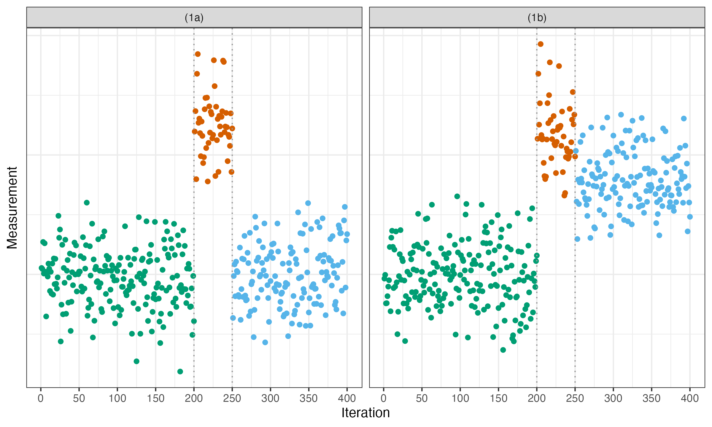
In both cases, we have a clear degradation at the 200th iteration and a clear acceleration at the 250th iteration. Most classic change point detectors easily detect both of these changes. When we detect such a short interval (shorter than a predefined threshold), we call it “temporary.” If there are several such intervals in a row, we join them into a single temporary interval. Therefore, there are no two subsequent temporary intervals: they are always separated by one of several long intervals that we call stable. The temporary intervals are not so interesting to research, so we want to condense the two corresponding change points into a single change event. However, not all the temporary intervals are equally interesting from the business perspective. Let us discuss two situations in the cases (1a) and (1b).
In the case (1a), the system was fully stabilized after a short period of degraded performance. We call it “temporary fluctuation.” Of course, the situation is suspicious: it may be worth considering researching why did this period happen. However, since the problem is fully gone, it is a kind of “important but not urgent” problem. I recommend silently adding it to the backlog of other suspicious cases deserving investigation. Of course, do not forget to assign some of your time to process this backlog. Systematic backlog processing is essential for building a reliable system. This allows better task prioritization and protects you from an overwhelming flow of incoming alerts.
The case (1b) definitely deserves more attention. Even though the last change point was an improvement, the system has not fully recovered after the previous degradation. We call such an interval “transition stage,” which can be also classified as degradation or acceleration. Here we observe a degradation-type transition stage: at the end, we still have worse performance than we had in the beginning.
Therefore, we have defined a business requirement: we want to distinguish temporary fluctuation (like (1a)) from transition stages (like (1b)) in our change point alert system.
The adjustment
There are plenty of existing change point detection algorithms. It will be too tedious to adapt all of them to support the distinguishing mechanism. Therefore, we suggest a postprocessing algorithm. Once the list of change points is obtained, we find all temporary intervals. In the cases (1a) and (1b), we suppose that both middle intervals are marked.
In the next stage, we cut the temporary intervals out and obtain the modified time series as shown below:
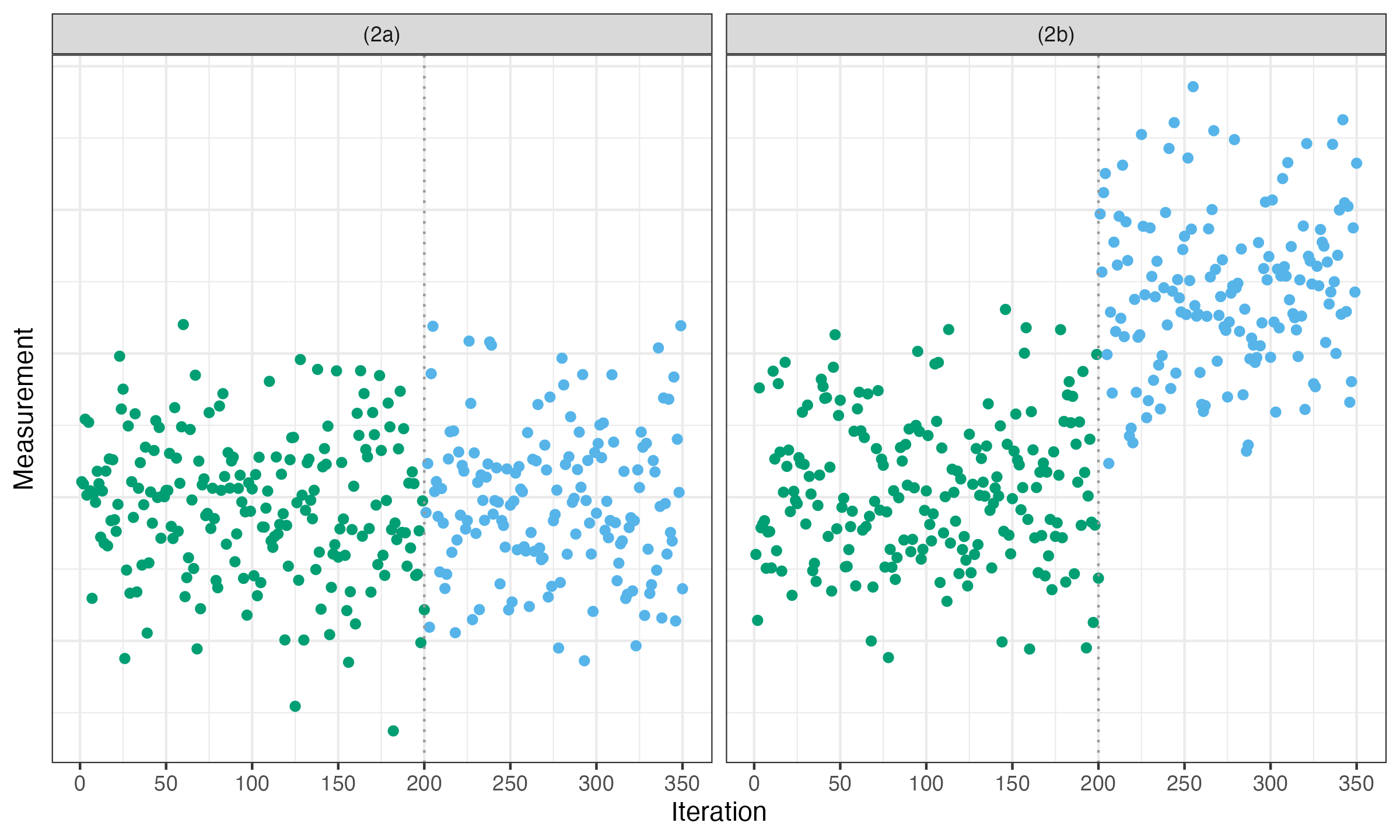
After that, we perform a second pass of the same change point detection algorithm but on the modified time series. If we detect a change point in the neighborhood of a cut point (say, half of the interval size threshold), the corresponding interval may be considered as a transition stage between two stable stages as in the case (2b). If there are no change points in the neighborhood of a cut point, the corresponding interval may be considered as a temporary fluctuation as in the case (2a).
Conclusion
The most reliable systems are typically designed with exceptional attention to detail. Some improvements may seem minor, but together they can significantly improve the overall system quality. Every single trick you apply to reduce the false-positive rate or improve the issue prioritization simplifies the life of the persons on duty and makes their happiness level higher.