Unbiased median absolute deviation based on the Harrell-Davis quantile estimator

The median absolute deviation ($\textrm{MAD}$) is a robust measure of scale. In the previous post, I showed how to use the unbiased version of the $\textrm{MAD}$ estimator as a robust alternative to the standard deviation. “Unbiasedness” means that such estimator’s expected value equals the true value of the standard deviation. Unfortunately, there is such thing as the bias–variance tradeoff: when we remove the bias of the $\textrm{MAD}$ estimator, we increase its variance and mean squared error ($\textrm{MSE}$).

In this post, I want to suggest a more efficient unbiased $\textrm{MAD}$ estimator. It’s also a consistent estimator for the standard deviation, but it has smaller $\textrm{MSE}$. To build this estimator, we should replace the classic “straightforward” median estimator with the Harrell-Davis quantile estimator and adjust bias-correction factors. Let’s discuss this approach in detail.

Introduction

Let’s consider a sample $x = \{ x_1, x_2, \ldots, x_n \}$. Its median absolute deviation $\textrm{MAD}_n$ can be defined as follows:

$$ \textrm{MAD}_n = C_n \cdot \textrm{median}(|X - \textrm{median}(X)|) $$

where $\textrm{median}$ is a median estimator, $C_n$ is a scale factor (or consistency constant).

Typically, $\textrm{median}$ assumes the classic “straightforward” median estimator:

• If $n$ is odd, the median is the middle element of the sorted sample
• If $n$ is even, the median is the arithmetic average of the two middle elements of the sorted sample

However, we can use other median estimators. Let’s consider $\textrm{median}_{\textrm{HD}}$ which calculates the median using the Harrell-Davis quantile estimator (see harrell1982):

$$ \textrm{median}_{\textrm{HD}}(x) = \sum_{i=1}^n W_i x_i, \quad W_i = I_{i/n} \bigg( \frac{n+1}{2}, \frac{n+1}{2} \bigg) - I_{(i-1)/n} \bigg( \frac{n+1}{2}, \frac{n+1}{2} \bigg) $$

where $I_t(a, b)$ denotes the regularized incomplete beta function.

When $n \to \infty$, we have the exact value of $C_n$ which makes $\textrm{MAD}_n$ an unbiased estimator for the standard deviation:

$$ C_n = C_\infty = \dfrac{1}{\Phi^{-1}(3/4)} \approx 1.4826022185056 $$

For finite values of $n$, we should use adjusted $C_n$ values. We already discussed these values for the straightforward median estimator in the previous post (this problem is well-covered in park2020). For $\textrm{median}_{\textrm{HD}}$, we should use another set of $C_n$ values. We reuse the approach from hayes2014 with the following notation:

$$ C_n = \dfrac{1}{\hat{a}_n} $$

Factors for small n

Factors for the small values of $n$ can be obtained using numerical experiments. Here is the scheme for the performed simulation:

• Enumerate $n$ from $2$ to $100$
• For each $n$, generate $2\cdot 10^8$ samples from the normal distribution of size $n$ (the Box–Muller transform is used, see [Box1958])
• For each sample, estimate $\textrm{MAD}_n$ using $C_n = 1$
• Calculate the arithmetic average of all $\textrm{MAD}_n$ values for the same $n$: the result is the value of $\hat{a}_n$

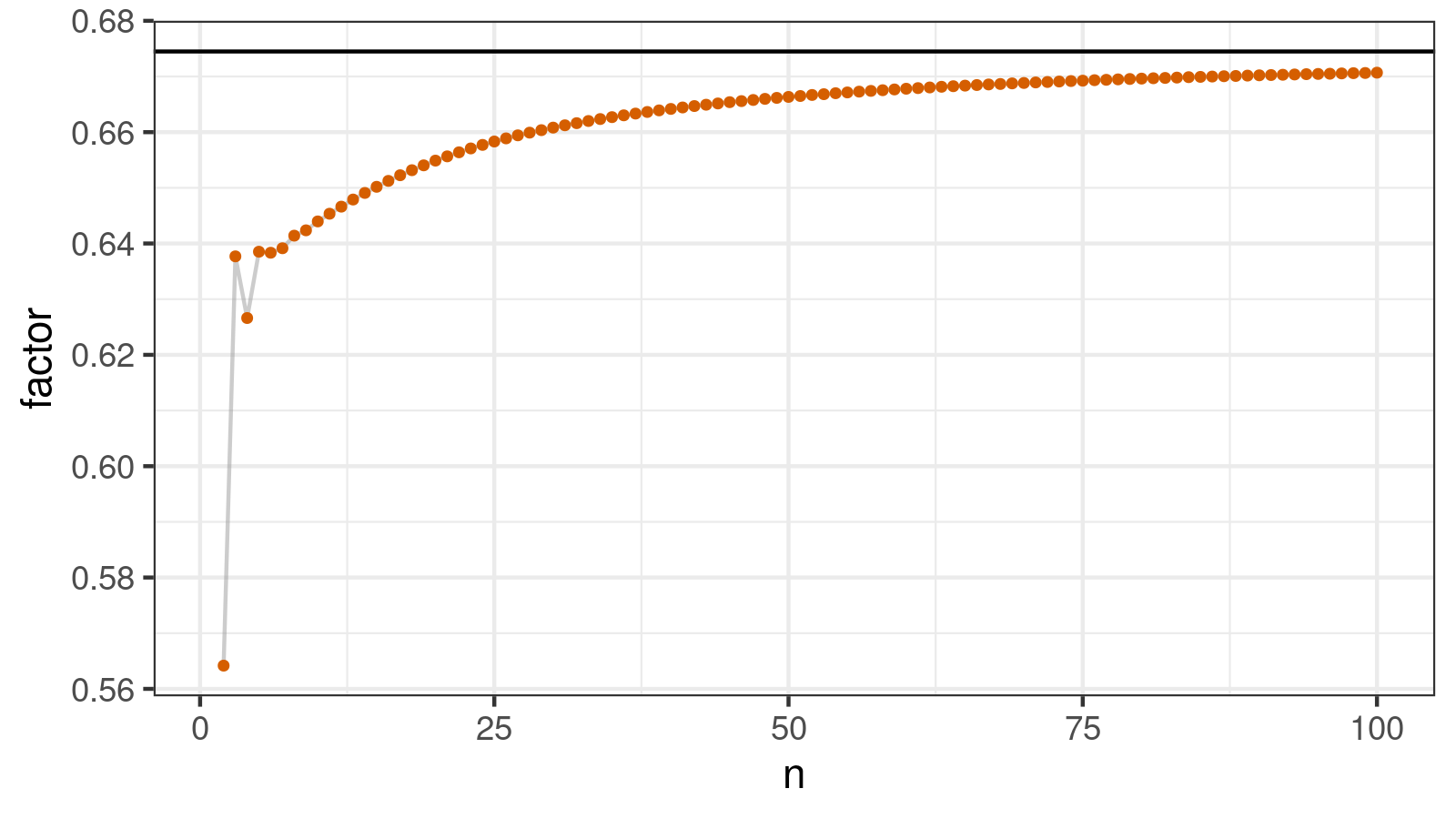
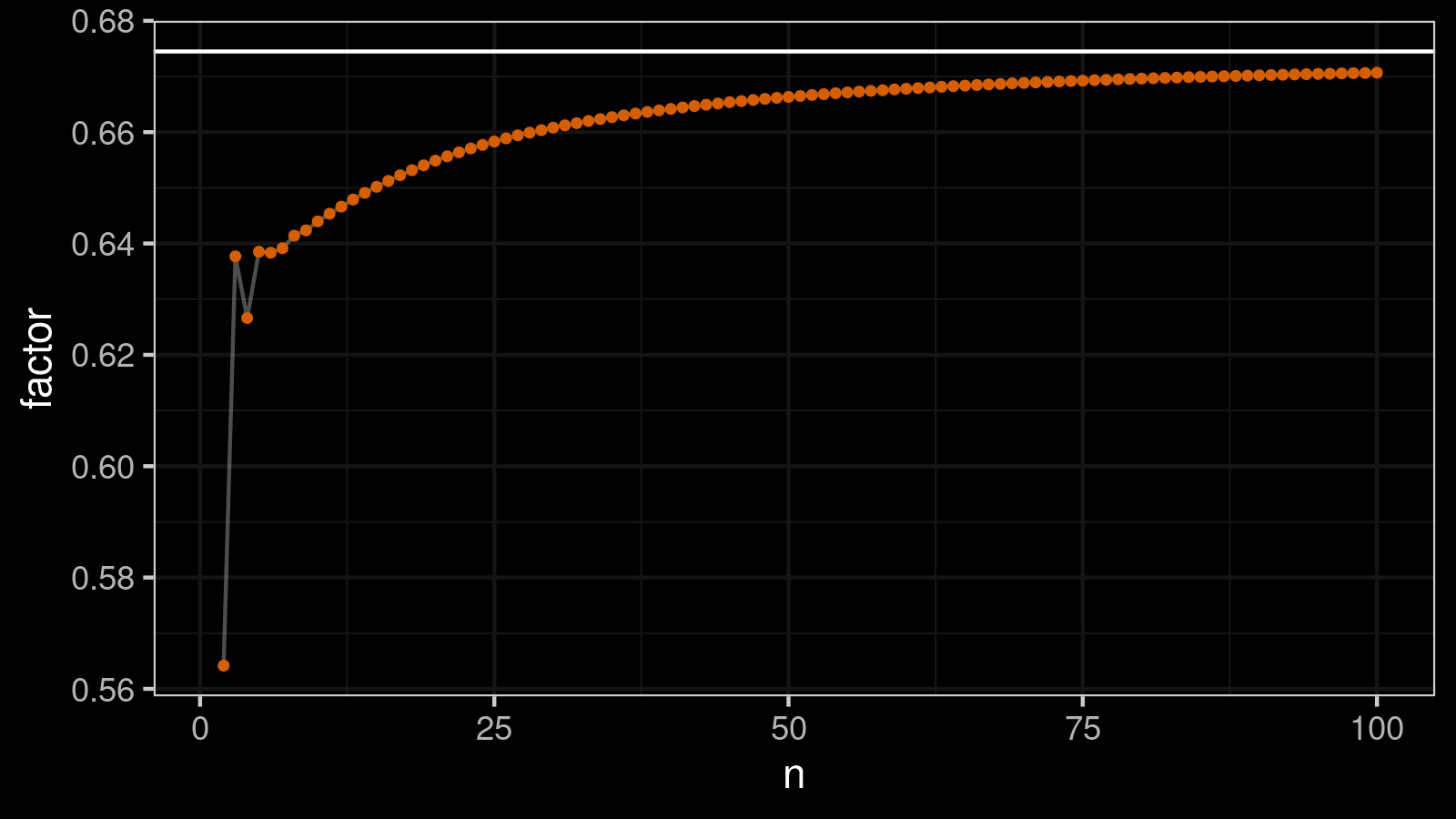
As the result of this simulation, I got the following table with $\hat{a}_n$ and $C_n$ values for $n \in \{ 2..100 \}$.

$n$	$\hat{a}_n$	$C_n$	$n$	$\hat{a}_n$	$C_n$
1	NA	NA	51	0.66649	1.50039
2	0.56417	1.77250	52	0.66668	1.49998
3	0.63769	1.56816	53	0.66682	1.49966
4	0.62661	1.59589	54	0.66699	1.49926
5	0.63853	1.56611	55	0.66713	1.49895
6	0.63834	1.56656	56	0.66728	1.49863
7	0.63915	1.56458	57	0.66741	1.49833
8	0.64141	1.55908	58	0.66753	1.49805
9	0.64237	1.55675	59	0.66767	1.49774
10	0.64397	1.55288	60	0.66780	1.49746
11	0.64535	1.54955	61	0.66791	1.49720
12	0.64662	1.54651	62	0.66803	1.49694
13	0.64790	1.54346	63	0.66815	1.49667
14	0.64908	1.54064	64	0.66825	1.49644
15	0.65018	1.53803	65	0.66836	1.49621
16	0.65125	1.53552	66	0.66846	1.49597
17	0.65226	1.53313	67	0.66857	1.49574
18	0.65317	1.53101	68	0.66865	1.49555
19	0.65404	1.52896	69	0.66876	1.49531
20	0.65489	1.52698	70	0.66883	1.49514
21	0.65565	1.52520	71	0.66893	1.49493
22	0.65638	1.52351	72	0.66901	1.49475
23	0.65708	1.52190	73	0.66910	1.49456
24	0.65771	1.52043	74	0.66918	1.49437
25	0.65832	1.51902	75	0.66925	1.49422
26	0.65888	1.51772	76	0.66933	1.49402
27	0.65943	1.51647	77	0.66940	1.49387
28	0.65991	1.51536	78	0.66948	1.49370
29	0.66036	1.51433	79	0.66955	1.49354
30	0.66082	1.51328	80	0.66962	1.49339
31	0.66123	1.51233	81	0.66968	1.49325
32	0.66161	1.51146	82	0.66974	1.49312
33	0.66200	1.51057	83	0.66980	1.49298
34	0.66235	1.50977	84	0.66988	1.49281
35	0.66270	1.50899	85	0.66993	1.49270
36	0.66302	1.50824	86	0.66999	1.49257
37	0.66334	1.50753	87	0.67005	1.49244
38	0.66362	1.50688	88	0.67009	1.49233
39	0.66391	1.50623	89	0.67016	1.49219
40	0.66417	1.50563	90	0.67021	1.49207
41	0.66443	1.50504	91	0.67026	1.49196
42	0.66469	1.50447	92	0.67031	1.49185
43	0.66493	1.50393	93	0.67036	1.49174
44	0.66515	1.50341	94	0.67041	1.49161
45	0.66539	1.50289	95	0.67046	1.49152
46	0.66557	1.50246	96	0.67049	1.49144
47	0.66578	1.50200	97	0.67055	1.49131
48	0.66598	1.50155	98	0.67060	1.49121
49	0.66616	1.50115	99	0.67063	1.49114
50	0.66633	1.50076	100	0.67068	1.49102

Here is a visualization of this table:

Factors for huge n

To build the equation for $n > 100$, we also continue the approach suggested in hayes2014 (pages 2208-2209) and use the prediction equation of the following form:

$$ \hat{a}_n = \Phi^{-1}(3/4) \Bigg( 1 - \dfrac{\alpha}{n} - \dfrac{\beta}{n^2} \Bigg). $$

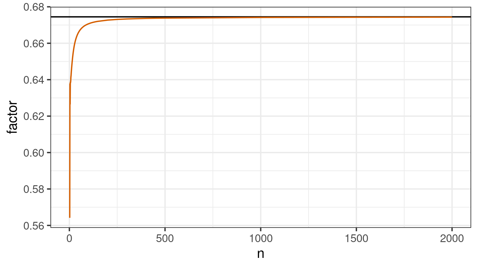
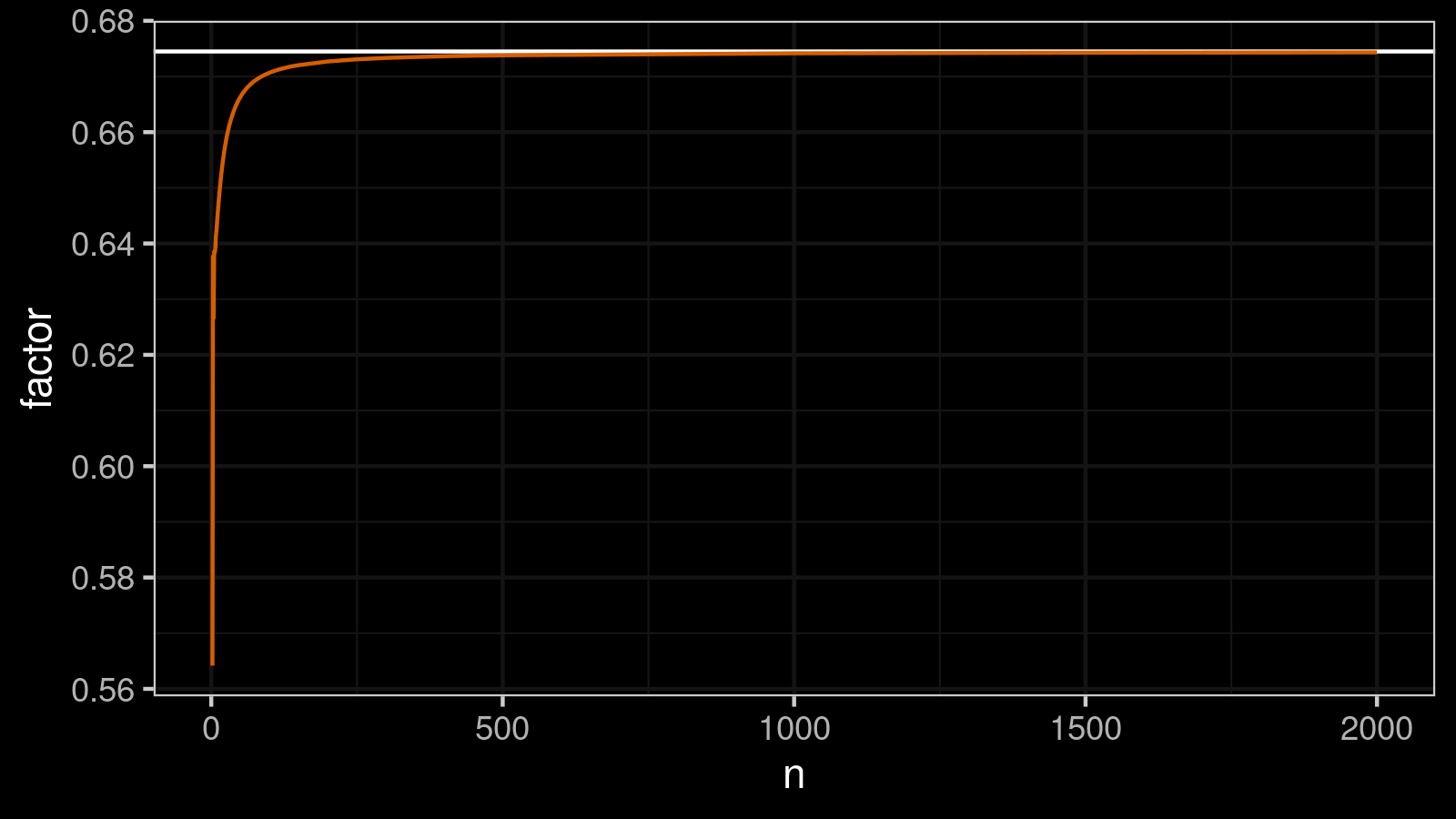
We simulated approximations of $\hat{a}_n$ for some large $n$ values:

$n$	$\hat{a}_n$
100	0.6707
110	0.6711
120	0.6714
130	0.6716
140	0.6719
150	0.6720
200	0.6727
250	0.6731
300	0.6733
350	0.6735
400	0.6736
450	0.6737
500	0.6738
1000	0.6742
1500	0.6743
2000	0.6743

Next, we fitted these values using the multiple linear regression. The dependent variable is $y = 1 - \hat{a}_n / \Phi^{-1}(3/4)$; the independent variables are $n^{-1}$ and $n^{-2}$; the intercept is zero:

$$ y = \alpha n^{-1} + \beta n^{-2}. $$

The fitted model was adjusted a little bit to get nice-looking values (keeping the good accuracy level):

$$ \alpha = 0.5,\quad \beta = 6.5. $$

These values give pretty accurate estimation of $\hat{a}_n$ for $n > 100$ (the accuracy is less than $10^{-4}$).

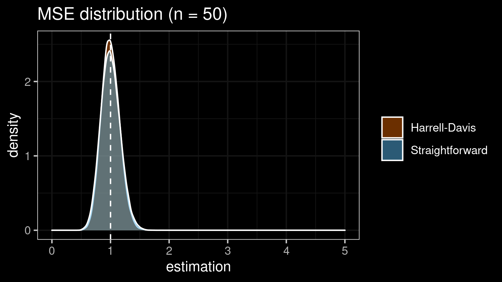
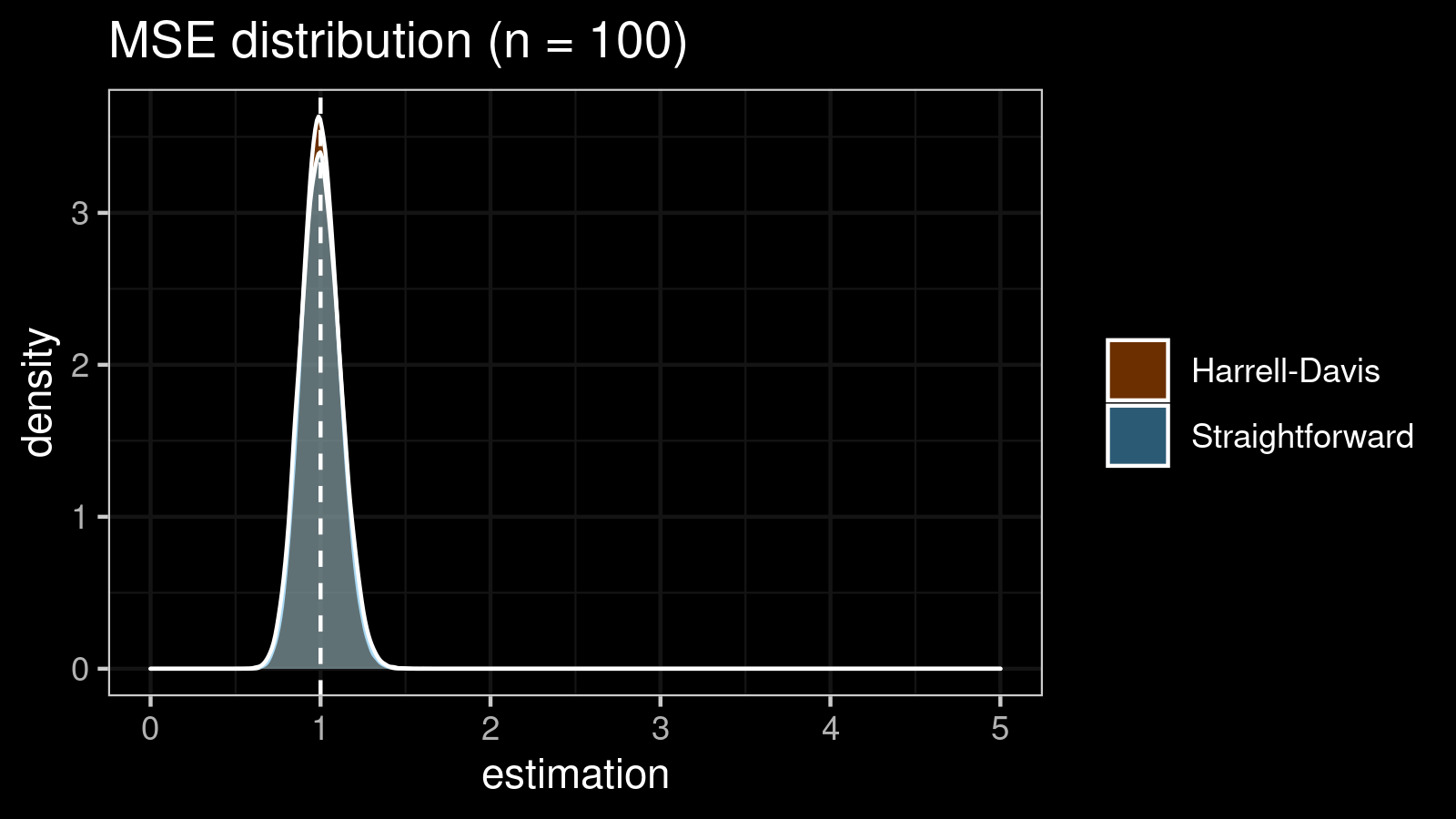
The mean squared error

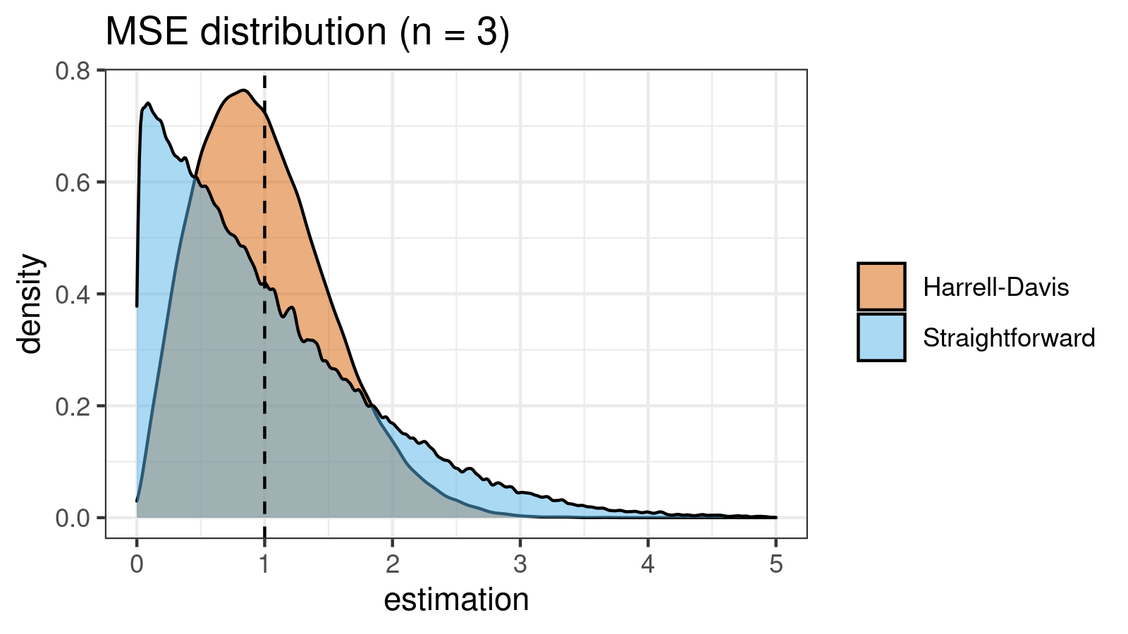
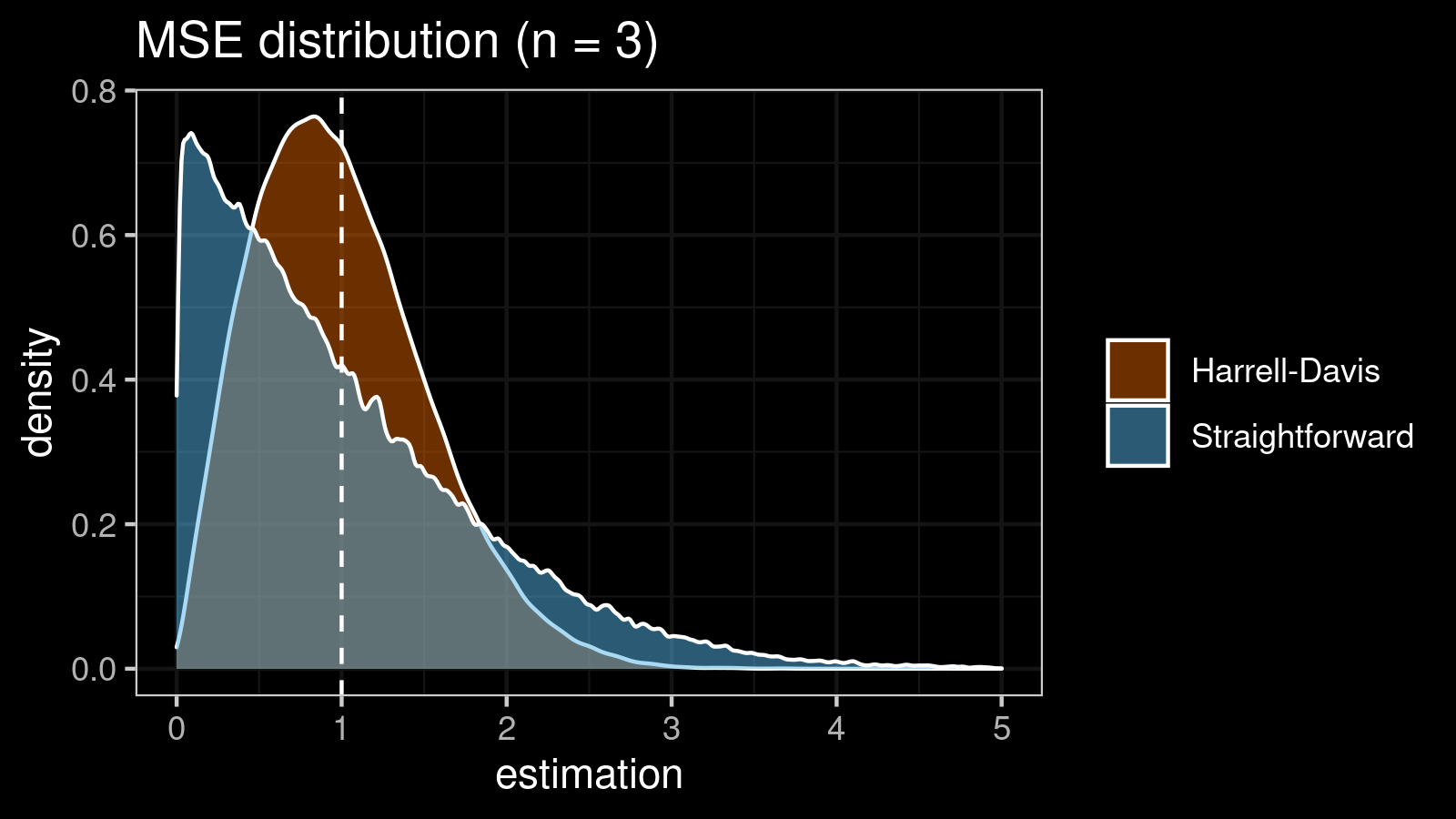
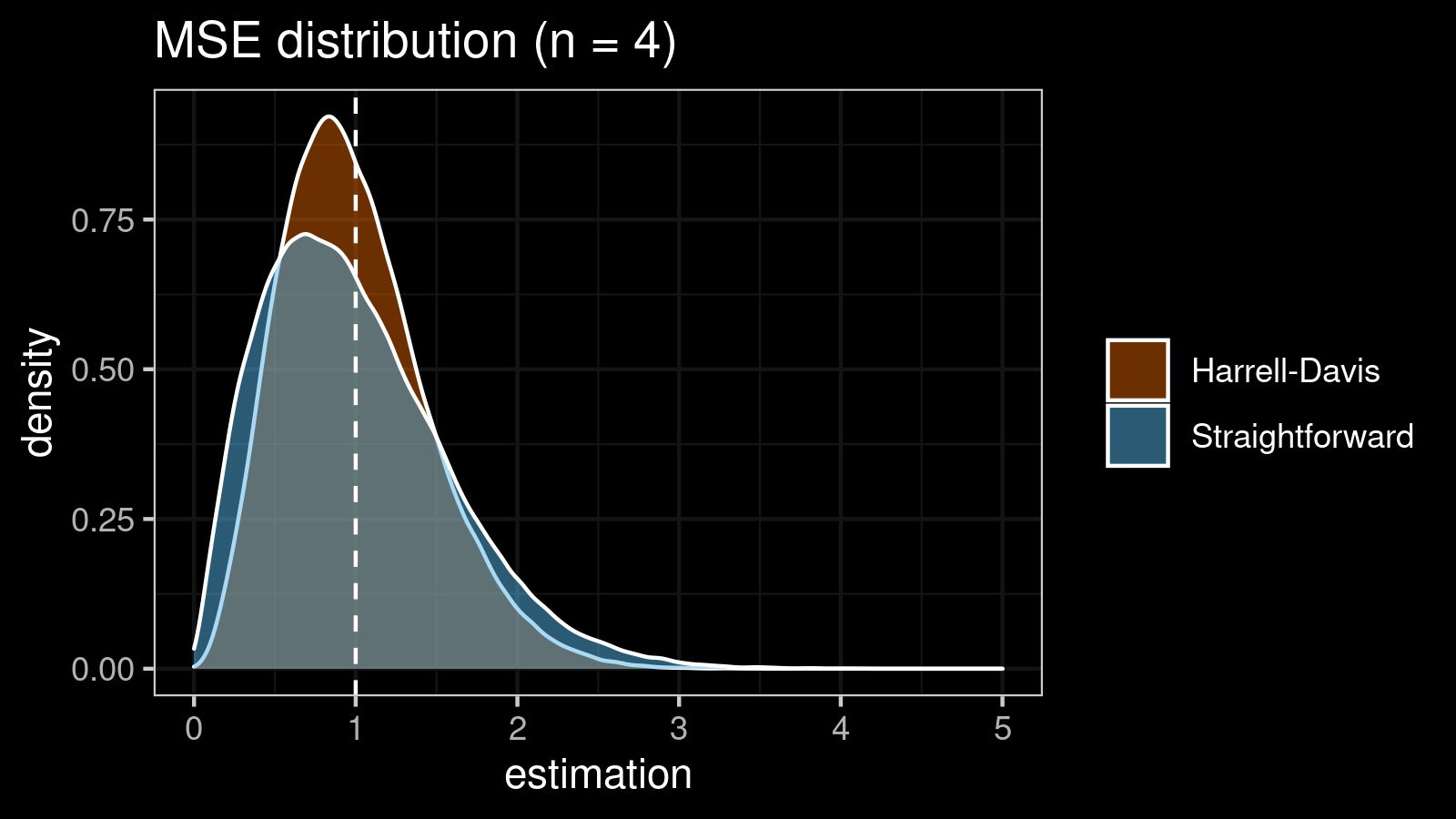
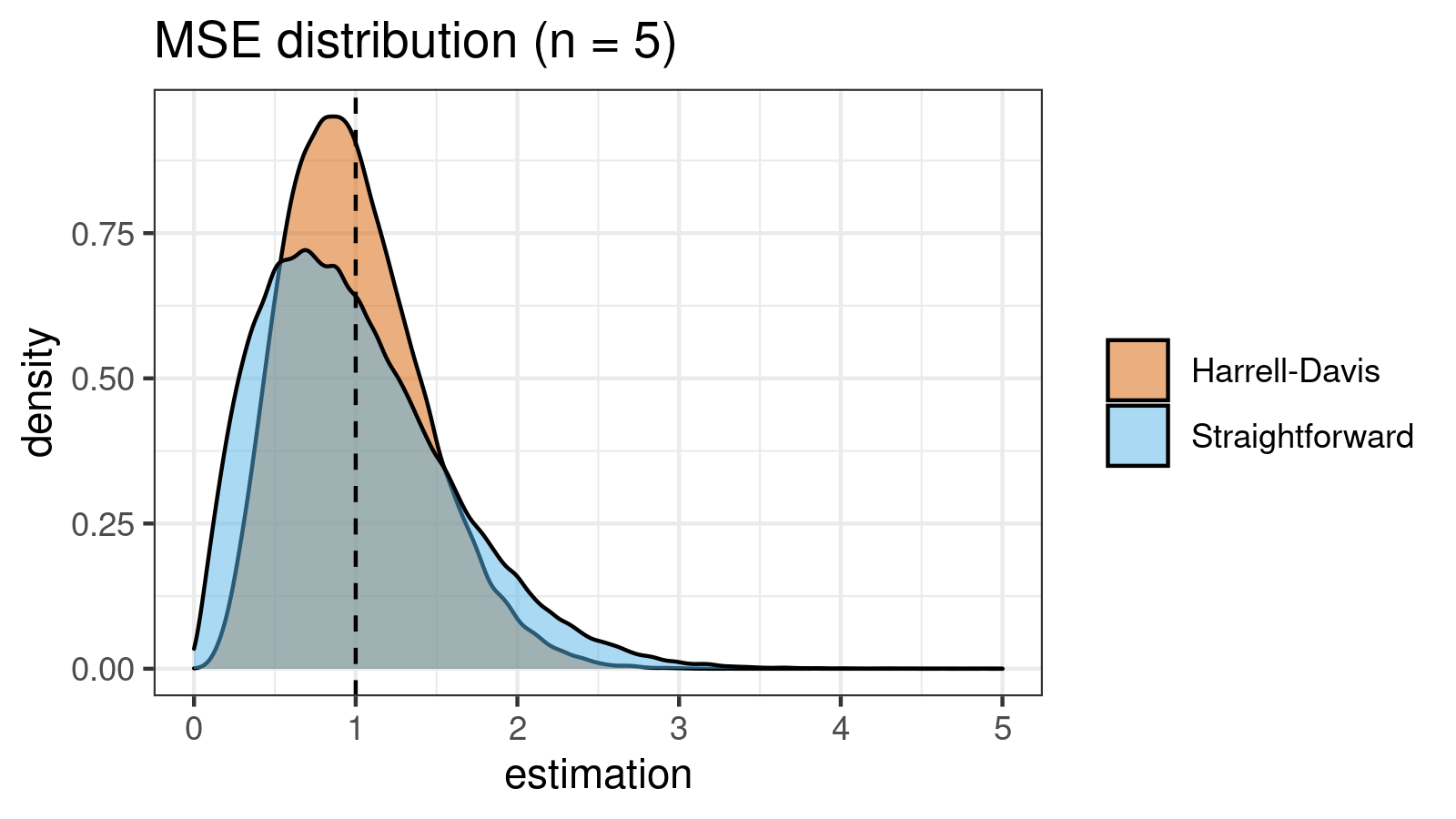
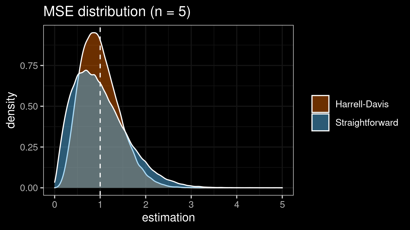
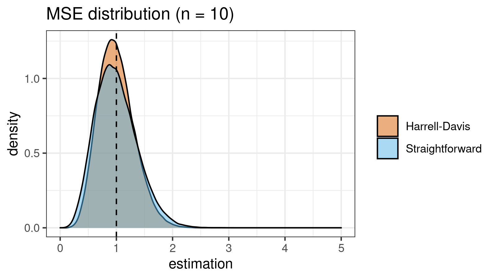
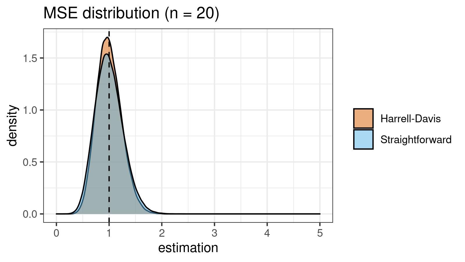
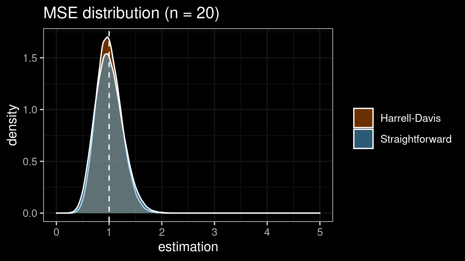
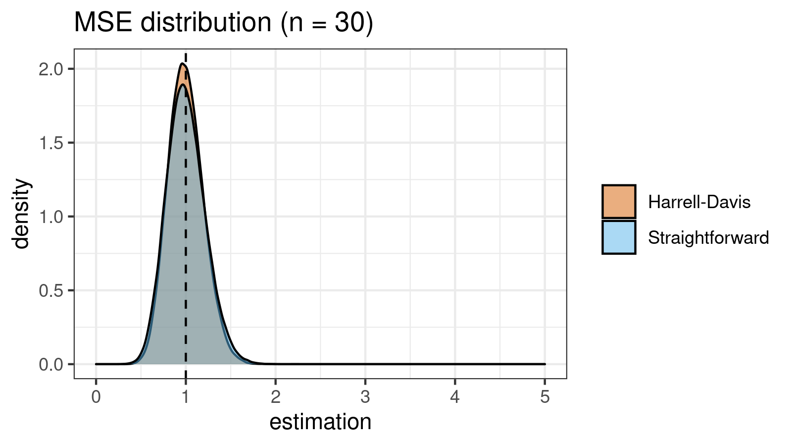
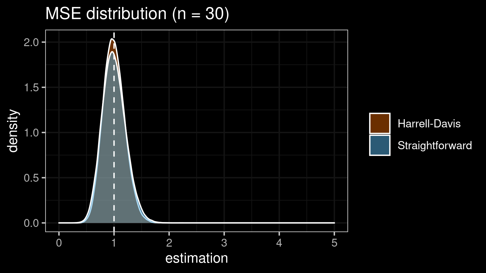
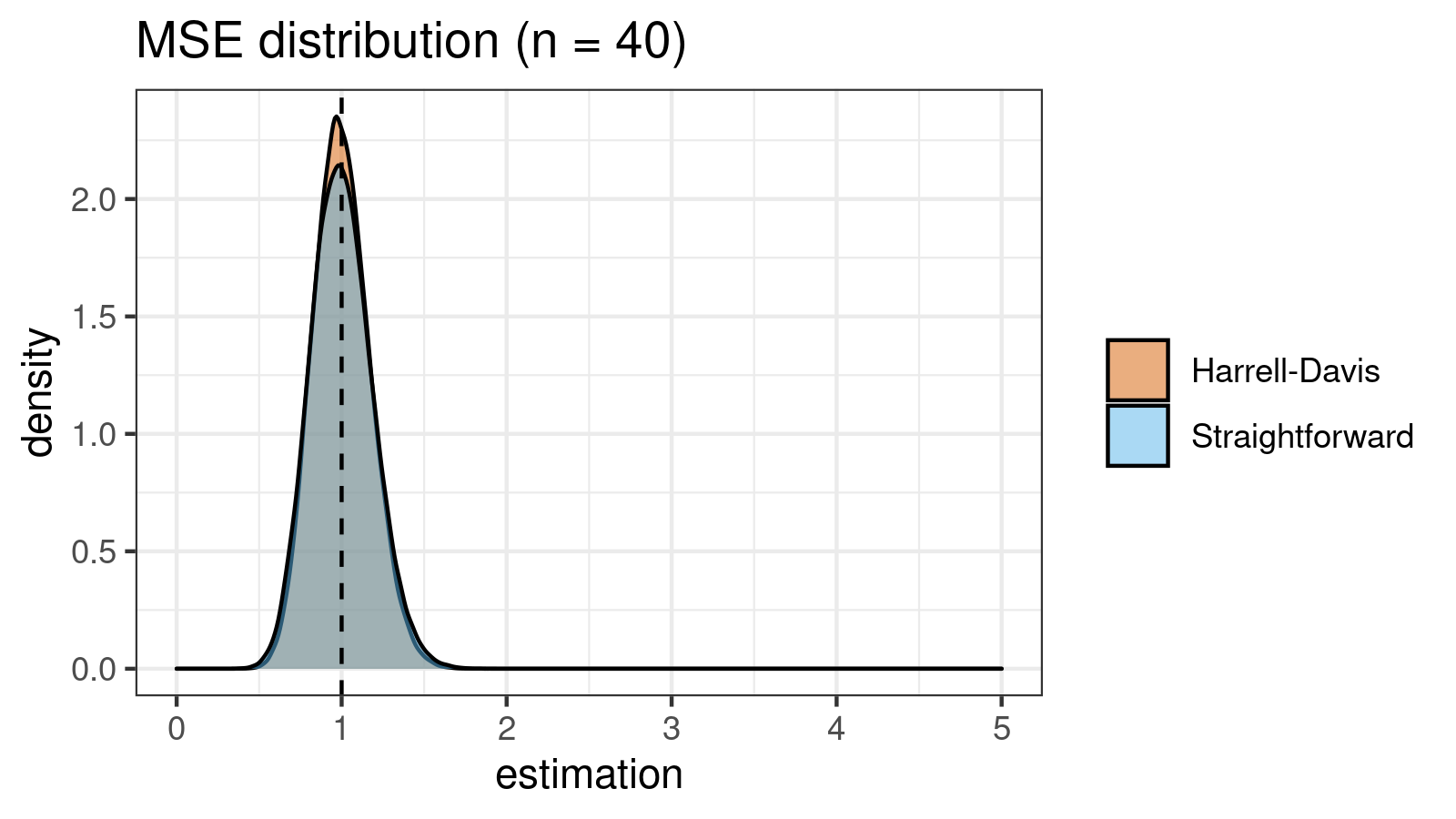
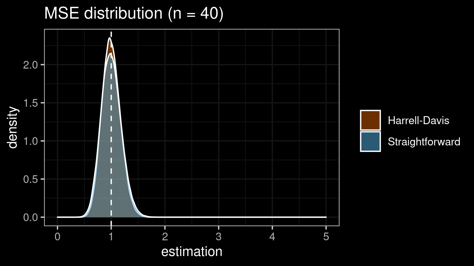
It’s time to compare the straightforward and the Harrell-Davis-based $\textrm{MAD}$ estimators in terms of the mean squared error. To estimate the $\textrm{MSE}$, we also use numerical simulations. Here are the results for some $n$ values:

n	Straightforward	Harrell-Davis
3	0.690	0.272
4	0.327	0.205
5	0.341	0.181
10	0.136	0.100
20	0.069	0.055
30	0.045	0.038
40	0.034	0.029
50	0.027	0.024
100	0.014	0.012

As we can see, the difference between estimators for small samples is tangible. For example, for $n = 3$, we got $\textrm{MSE} \approx 0.69$ for the straightforward estimator vs. $\textrm{MSE} \approx 0.27$ for the Harrell-Davis-based estimator. Below you can see density plots of $\textrm{MSE}$ for the above $n$ values.

Conclusion

In this post, we discussed the unbiased $\textrm{MAD}_n$ estimator which is based on the Harrell-Davis quantile estimator instead of the straightforward median estimator. The suggested estimator is much more efficient for small samples because it has smaller $\textrm{MSE}$. It allows using $\textrm{MAD}_n$ as a efficient alternative to the standard deviation under the normal distribution with higher accuracy.

References

• [Harrell1982]
  Harrell, F.E. and Davis, C.E., 1982. A new distribution-free quantile estimator. Biometrika, 69(3), pp.635-640.
  https://doi.org/10.2307/2335999
• [Hayes2014]
  Hayes, Kevin. “Finite-sample bias-correction factors for the median absolute deviation.” Communications in Statistics-Simulation and Computation 43, no. 10 (2014): 2205-2212.
  https://doi.org/10.1080/03610918.2012.748913
• [Park2020]
  Park, Chanseok, Haewon Kim, and Min Wang. “Investigation of finite-sample properties of robust location and scale estimators.” Communications in Statistics-Simulation and Computation (2020): 1-27.
  https://doi.org/10.1080/03610918.2019.1699114
• [Box1958]
  Box, George EP. “A note on the generation of random normal deviates.” Ann. Math. Statist. 29 (1958): 610-611.
  https://doi.org/10.1214/aoms/1177706645