Unbiased median absolute deviation based on the trimmed Harrell-Davis quantile estimator

The median absolute deviation ($\operatorname{MAD}$) is a robust measure of scale. For a sample $x = \{ x_1, x_2, \ldots, x_n \}$, it’s defined as follows:

$$ \operatorname{MAD}_n = C_n \cdot \operatorname{median}(|x - \operatorname{median}(x)|) $$

where $\operatorname{median}$ is a median estimator, $C_n$ is a scale factor. Using the right scale factor, we can use $\operatorname{MAD}$ as a consistent estimator for the estimation of the standard deviation under the normal distribution. For huge samples, we can use the asymptotic value of $C_n$ which is

$$ C_\infty = \dfrac{1}{\Phi^{-1}(3/4)} \approx 1.4826022185056. $$

For small samples, we should use adjusted values $C_n$ which depend on the sample size. However, $C_n$ depends not only on the sample size but also on the median estimator. I have already covered how to obtain this values for the traditional median estimator and the Harrell-Davis median estimator. It’s time to get the $C_n$ values for the trimmed Harrell-Davis median estimator.

Simulation

In order to obtain the values of $C_n$, we perform the following simulation:

• Enumerate $n$ from $2$ to $100$ and some other values up to $2000$.
• For each $n$, generate $2\cdot 10^8$ samples from the normal distribution of size $n$ (the Box–Muller transform is used, see [Box1958])
• For each sample, estimate $\textrm{MAD}_n$ using $C_n = 1$ and the trimmed Harrell-Davis quantile estimator based on the highest density interval of the width $1/sqrt(n)$ (aka THD-SQRT).
• Calculate the arithmetic average of all $\textrm{MAD}_n$ values for the same $n$: the result is the value of $\hat{a}_n$
• The reverse value is the estimation of $C_n = 1/\hat{a}_n$.

Warning: on my PC, the simulation takes several days to finish.

Results for small n

Here are the results for $n \leq 100$:

n	$C_n$
2	1.7724370908056342
3	1.6455078173901185
4	2.017065193495793
5	1.6774358847728241
6	1.6886228884833927
7	1.681012890164465
8	1.6363164157283878
9	1.6430595153542609
10	1.6137117695811252
11	1.6036656575624237
12	1.5938702075534783
13	1.5826054249267754
14	1.5770618699717638
15	1.568314144069548
16	1.5639360738331398
17	1.5574345825637932
18	1.5530068367429388
19	1.548786644010622
20	1.5449266898438678
21	1.5417268298909585
22	1.5385447997218455
23	1.5360433134061504
24	1.5333044878734197
25	1.5313026814346553
26	1.5289087814370173
27	1.5271766811326293
28	1.525372045244657
29	1.523823710130717
30	1.5223707036738177
31	1.5210003444944378
32	1.5198014780734148
33	1.5185318176366789
34	1.5174778699831464
35	1.5163204121308342
36	1.515455864530263
37	1.514367919034956
38	1.5135668482892533
39	1.512646068257695
40	1.5119358224536255
41	1.5111386979568142
42	1.5104143980692895
43	1.5097598792706493
44	1.5090605208097354
45	1.5085030887342528
46	1.5078365336949058
47	1.5073406253974977
48	1.506750314567103
49	1.5063216542860618
50	1.5056976215756004
51	1.5052645904785493
52	1.5047506790429501
53	1.504377980905483
54	1.5039313123542895
55	1.5035247994299705
56	1.5031546583298019
57	1.5027213700422273
58	1.5023816126090916
59	1.501979658633948
60	1.5016812388186662
61	1.5013235911210157
62	1.5010571020037526
63	1.5006852968235684
64	1.5004714716576355
65	1.5001142465452528
66	1.4998450017251428
67	1.4995612278126766
68	1.4993166731144414
69	1.499031830812627
70	1.498806802914833
71	1.4985656090426709
72	1.498311085994739
73	1.4980998089801867
74	1.4978614270801778
75	1.4976461613303127
76	1.497450811659424
77	1.4972614163628544
78	1.497019612065497
79	1.496874216833877
80	1.4966283982987492
81	1.4964878123374772
82	1.4962757052242632
83	1.496149471166867
84	1.4959392546341381
85	1.4957683906834602
86	1.4956060922384664
87	1.4954645049047413
88	1.495307563560535
89	1.4951503339020875
90	1.49500530886384
91	1.4948486175521838
92	1.494716574686503
93	1.4946021151410946
94	1.4944505753829063
95	1.4942998891427248
96	1.494198277219056
97	1.4940563287162394
98	1.4939476227923159
99	1.493783721728854
100	1.4937221140129977

Results for huge n

I have also calculated $C_n$ for some bigger sample sizes:

n	$C_n$
100	1.4937221140129977
110	1.492629467879562
120	1.491756950186543
130	1.4910176116133274
140	1.4903922085488397
150	1.4898464598871315
200	1.487963070934298
250	1.4868507636216115
300	1.4861201577554497
350	1.4855909210465295
400	1.4852251546501989
450	1.4849172381877342
500	1.4846796356493557
1000	1.4836281802634783
1500	1.4832857748830472
2000	1.4831139879531638
2500	1.4830091511037906
3000	1.4829398344041957
3500	1.4828931807149206
4000	1.4828555508375267
4500	1.4828287173605137

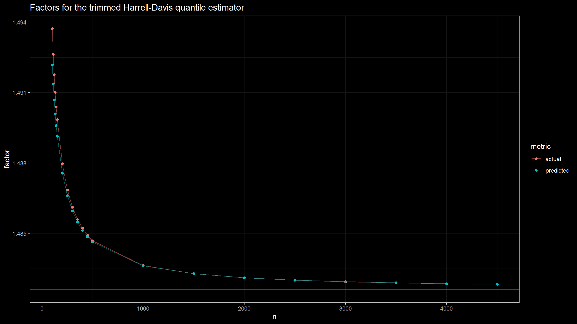
Following the approach from Investigation of finite-sample properties of robust location and scale estimators
By Chanseok Park, Haewon Kim, Min Wang · 2020park2020, we express $C_n$ using the following equation:

$$ C_n = \frac{1}{\Phi^{-1}(3/4) \cdot (1 - \alpha / n - \beta / n^2)} $$

With the help of linear regression, we get the following values of $\alpha$ and $beta$:

$$ \alpha \approx 0.69, \quad \beta = 5.14. $$

Here is a plot with both actual and predicted values of $C_n$ for different sample sizes:

References

• [Box1958]
  Box, George EP. “A note on the generation of random normal deviates.” Ann. Math. Statist. 29 (1958): 610-611.
  https://doi.org/10.1214/aoms/1177706645
• [Park2020]
  Park, Chanseok, Haewon Kim, and Min Wang. “Investigation of finite-sample properties of robust location and scale estimators.” Communications in Statistics-Simulation and Computation (2020): 1-27.
  https://doi.org/10.1080/03610918.2019.1699114