Unbiased median absolute deviation

The median absolute deviation ($\textrm{MAD}$) is a robust measure of scale. For distribution $X$, it can be calculated as follows:

$$ \textrm{MAD} = C \cdot \textrm{median}(|X - \textrm{median}(X)|) $$

where $C$ is a constant scale factor. This metric can be used as a robust alternative to the standard deviation. If we want to use the $\textrm{MAD}$ as a consistent estimator for the standard deviation under the normal distribution, we should set

$$ C = C_{\infty} = \dfrac{1}{\Phi^{-1}(3/4)} \approx 1.4826022185056. $$

where $\Phi^{-1}$ is the quantile function of the standard normal distribution (or the inverse of the cumulative distribution function). If $X$ is the normal distribution, we get $\textrm{MAD} = \sigma$ where $\sigma$ is the standard deviation.

Now let’s consider a sample $x = \{ x_1, x_2, \ldots x_n \}$. Let’s denote the median absolute deviation for a sample of size $n$ as $\textrm{MAD}_n$. The corresponding equation looks similar to the definition of $\textrm{MAD}$ for a distribution:

$$ \textrm{MAD}_n = C_n \cdot \textrm{median}(|x - \textrm{median}(x)|). $$

Let’s assume that $\textrm{median}$ is the straightforward definition of the median (if $n$ is odd, the median is the middle element of the sorted sample, if $n$ is even, the median is the arithmetic average of the two middle elements of the sorted sample). We still can use $C_n = C_{\infty}$ for extremely large sample sizes. However, for small $n$, $\textrm{MAD}_n$ becomes a biased estimator. If we want to get an unbiased version, we should adjust the value of $C_n$.

In this post, we look at the possible approaches and learn the way to get the exact value of $C_n$ that makes $\textrm{MAD}_n$ unbiased estimator of the median absolute deviation for any $n$.

The bias

Let’s briefly discuss the impact of the bias on our measurements. To illustrate the problem, we take $100\,000$ samples of size $n = 5$ from the standard normal distribution and calculate $\textrm{MAD}_5$ for each of them using $C = 1$. The obtained numbers form the following distribution:

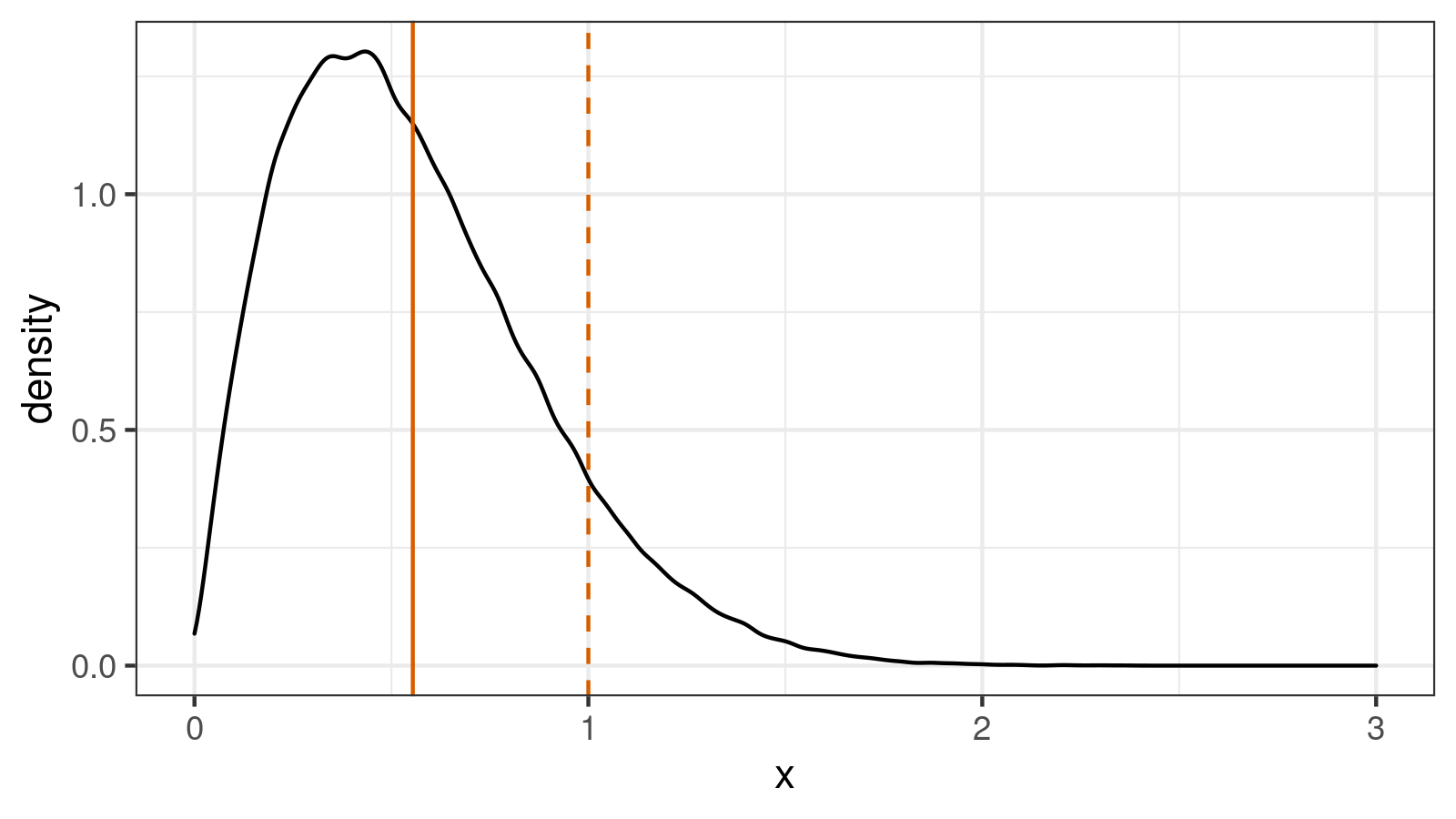
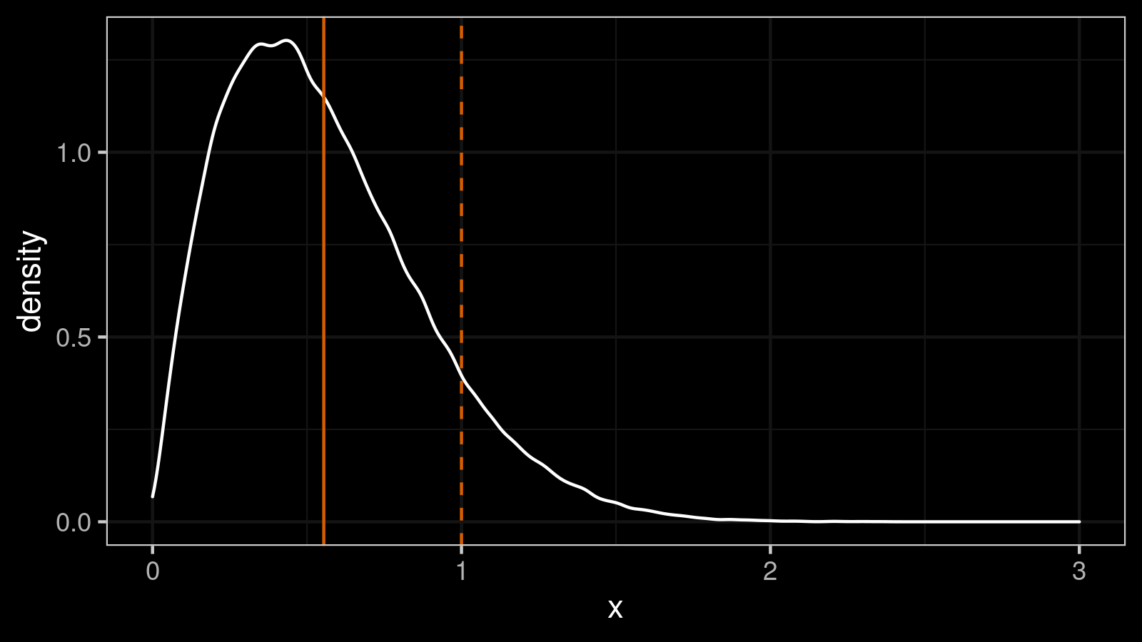
If we try to use $\textrm{MAD}_5$ with $C = 1$ as a standard deviation estimator, it would be a biased estimator. Indeed, the standard deviation equals $1$ (the true value), but the expected value of $\textrm{MAD}_5$ is about $E[\textrm{MAD}_5] \approx 0.5542$. In order to make it unbiased, we should set $C_5 = 1 / 0.5542 \approx 1.804$. If we repeat the experiment with the modified scale factor, we get a modified version of our distribution:

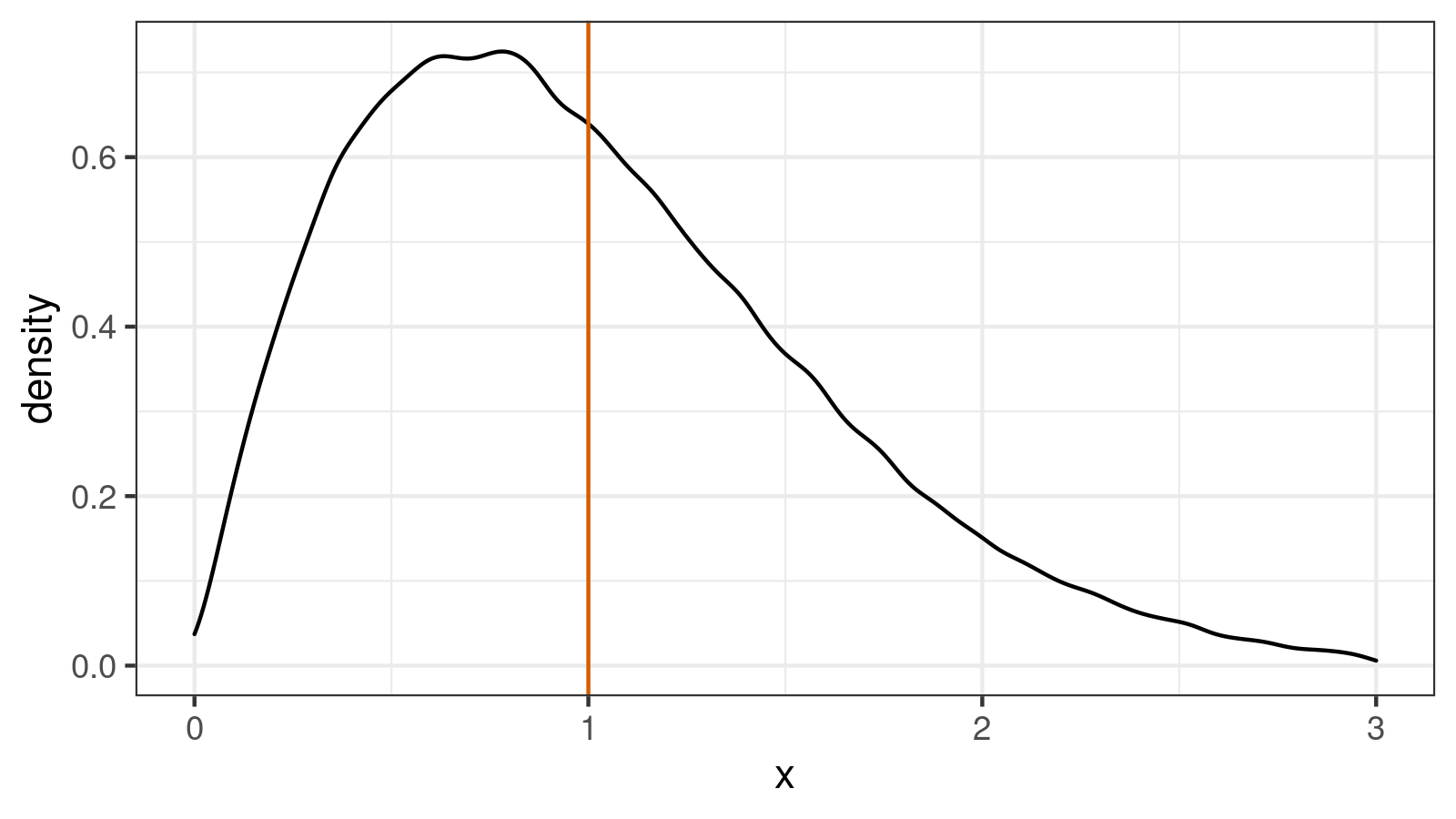
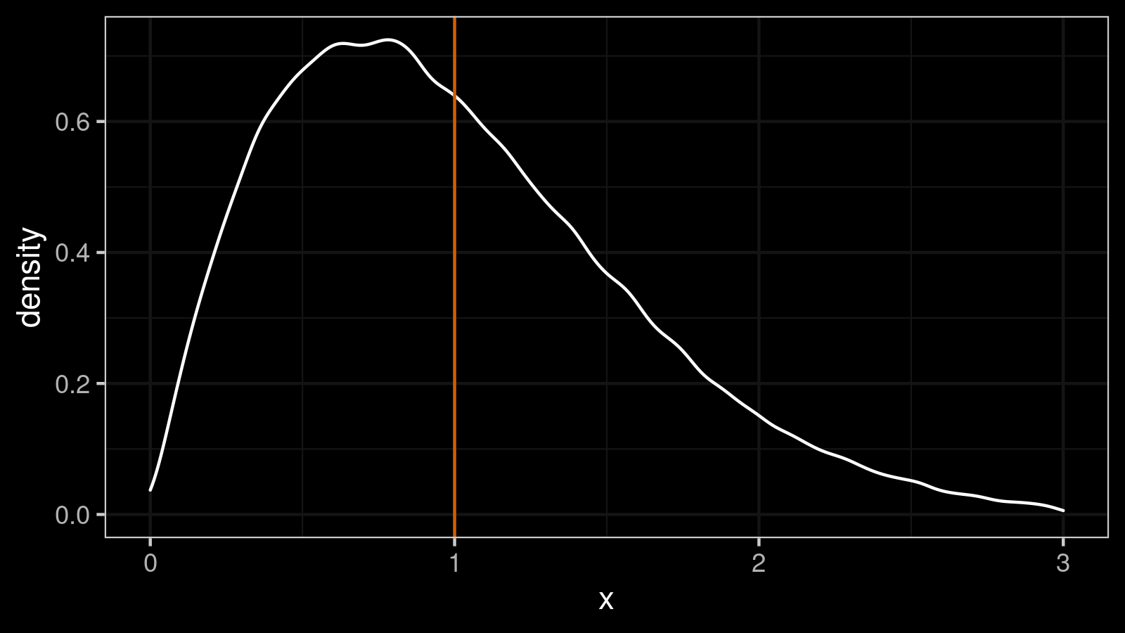
Now $E[\textrm{MAD}_5] \approx 1$ which makes $\textrm{MAD}_5$ unbiased estimator.

Note that $C_5 = 1.804$ differs from $C_{\infty} \approx 1.4826$ which is the proper scale factor for $n \to \infty$. Each sample size needs its own scale factor to make $\textrm{MAD}_n$ unbiased. Let’s review some papers and look at different approaches to find the optimal scale factor value.

Literature overview

One of the first mentions of the median absolute deviation can be found in hampel1974. In this paper, Frank R Hampel introduced $\textrm{MAD}$ as a robust measure of scale (attributed to Gauss). I have found four papers that describe unbiased versions: croux1992, williams2011, hayes2014, and park2020. Let’s briefly discuss approaches from these papers.

The Croux-Rousseeuw approach

In croux1992, Christophe Croux and Peter J. Rousseeuw described an unbiased version of $\textrm{MAD}$. They suggested using the following equations:

$$ C_n = \dfrac{b_n}{\Phi^{-1}(3/4)}. $$

For $n \leq 9$, the approximated values of $b_n$ were defined as follows:

n	$b_n$
2	1.196
3	1.495
4	1.363
5	1.206
6	1.200
7	1.140
8	1.129
9	1.107

For $n > 9$, they suggested to use the following equation:

$$ b_n = \dfrac{n}{n-0.8}. $$

The Williams approach

In williams2011, Dennis C. Williams improved this approach. Firstly, he provided updated $b_n$ values for small $n$:

n	$b_n$ by Croux	$b_n$ by Williams
2	1.196	1.197
3	1.495	1.490
4	1.363	1.360
5	1.206	1.217
6	1.200	1.189
7	1.140	1.138
8	1.129	1.127
9	1.107	1.101

Secondly, he also introduced a small correction for the general equation:

$$ b_n = \dfrac{n}{n-0.801}. $$

Also, he discussed another kind of approximation equation for such kind of bias-correction factors:

$$ b_n \cong 1 + cn^{-d}. $$

In his paper, he applied the above equation only to Shorth (which is the smallest interval that contains at least half of the data points), but this approach can also be applied to other measures of scale.

The Hayes approach

Next, in hayes2014, Kevin Hayes suggested another kind of prediction equation for $n \geq 9$:

$$ C_n = \dfrac{1}{\hat{a}_n} $$

where

$$ \hat{a}_n = \Phi^{-1}(3/4) \Bigg( 1 - \dfrac{\alpha}{n} - \dfrac{\beta}{n^2} \Bigg). $$

Here are the suggested constants:

n	$\alpha$	$\beta$
odd	0.7635	0.565
even	0.7612	1.123

The Park-Kim-Wang approach

Finally, in park2020, Chanseok Park, Haewon Kim, and Min Wang aggregated all of the previous results. They used the following form of the main equation:

$$ C_n = \dfrac{1}{\Phi^{-1}(3/4) \cdot (1+A_n)} $$

For $n > 100$, they suggested two approaches. The first one is based on hayes2014 (the same equation for both odd and even $n$ values):

$$ A_n = -\dfrac{0.76213}{n} - \dfrac{0.86413}{n^2} $$

The second one is based on williams2011:

$$ A_n = -0.804168866 \cdot n^{-1.008922} $$

Both approaches produce almost identical results, so it doesn’t actually matter which one to use.

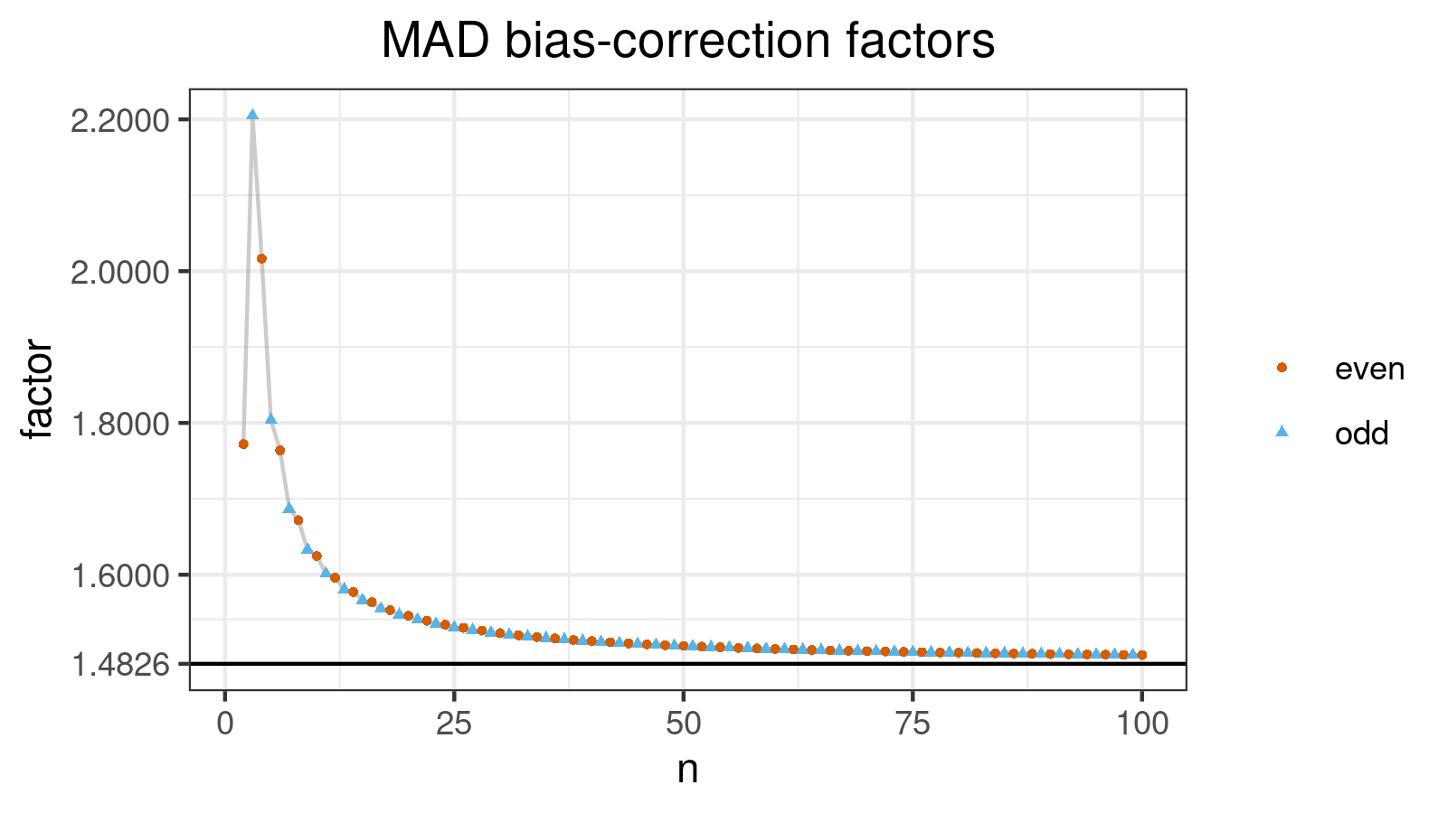
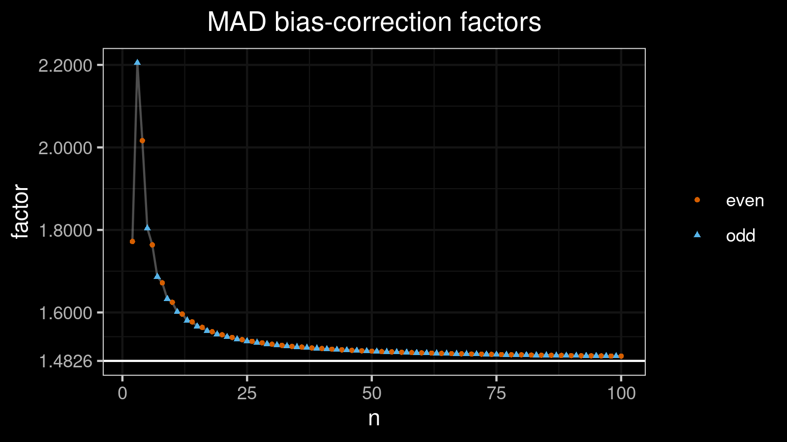
For $2 \leq n \leq 100$, they suggested to use predefined constants: (the below values are based on Table A2 from park2020):

n	$C_n$	n	$C_n$
1	NA	51	1.505611
2	1.772150	52	1.505172
3	2.204907	53	1.504575
4	2.016673	54	1.504417
5	1.803927	55	1.503713
6	1.763788	56	1.503604
7	1.686813	57	1.503095
8	1.671843	58	1.502864
9	1.632940	59	1.502253
10	1.624681	60	1.502085
11	1.601308	61	1.501611
12	1.596155	62	1.501460
13	1.580754	63	1.501019
14	1.577272	64	1.500841
15	1.566339	65	1.500331
16	1.563769	66	1.500343
17	1.555284	67	1.499877
18	1.553370	68	1.499772
19	1.547206	69	1.499291
20	1.545705	70	1.499216
21	1.540681	71	1.498922
22	1.539302	72	1.498838
23	1.535165	73	1.498491
24	1.534053	74	1.498399
25	1.530517	75	1.497917
26	1.529996	76	1.497901
27	1.526916	77	1.497489
28	1.526422	78	1.497544
29	1.523608	79	1.497248
30	1.523031	80	1.497185
31	1.520732	81	1.496797
32	1.520333	82	1.496779
33	1.518509	83	1.496428
34	1.517941	84	1.496501
35	1.516279	85	1.496295
36	1.516070	86	1.496089
37	1.514425	87	1.495794
38	1.513989	88	1.495796
39	1.512747	89	1.495557
40	1.512418	90	1.495420
41	1.511078	91	1.495270
42	1.511041	92	1.495141
43	1.509858	93	1.494944
44	1.509499	94	1.494958
45	1.508529	95	1.494706
46	1.508365	96	1.494665
47	1.507535	97	1.494379
48	1.507247	98	1.494331
49	1.506382	99	1.494113
50	1.506307	100	1.494199

Here is the corresponding plot:

Conclusion

Currently, my tool-of-choice is the approach from park2020]. I verified all the predefined constants and equations from the paper using numerical simulations. I can confirm that the suggested approach produces a reliable estimate of the unbiased median absolute deviation $\textrm{MAD}_n$.

References

• [Hampel1974]
  Hampel, Frank R. “The influence curve and its role in robust estimation.” Journal of the american statistical association 69, no. 346 (1974): 383-393.
  https://doi.org/10.2307/2285666
• [Croux1992]
  Croux, Christophe, and Peter J. Rousseeuw. “Time-efficient algorithms for two highly robust estimators of scale.“In Computational statistics, pp. 411-428. Physica, Heidelberg, 1992.
  https://doi.org/10.1007/978-3-662-26811-7_58
• [Williams2011]
  Williams, Dennis C. “Finite sample correction factors for several simple robust estimators of normal standard deviation.” Journal of Statistical Computation and Simulation 81, no. 11 (2011): 1697-1702.
  https://doi.org/10.1080/00949655.2010.499516
• [Hayes2014]
  Hayes, Kevin. “Finite-sample bias-correction factors for the median absolute deviation.” Communications in Statistics-Simulation and Computation 43, no. 10 (2014): 2205-2212.
  https://doi.org/10.1080/03610918.2012.748913
• [Park2020]
  Park, Chanseok, Haewon Kim, and Min Wang. “Investigation of finite-sample properties of robust location and scale estimators.” Communications in Statistics-Simulation and Computation (2020): 1-27.
  https://doi.org/10.1080/03610918.2019.1699114