Weighted Hodges-Lehmann location estimator and mixture distributions

The classic non-weighted Hodges-Lehmann EstimatorHodges-Lehmann location estimator of a sample $\mathbf{x} = (x_1, x_2, \ldots, x_n)$ is defined as follows:

$$ \operatorname{HL}(\mathbf{x}) = \underset{1 \leq i \leq j \leq n}{\operatorname{median}} \left(\frac{x_i + x_j}{2} \right), $$

where $\operatorname{median}$ is the sample median. Previously, we have defined a weighted version of the Hodges-Lehmann location estimator as follows:

$$ \operatorname{WHL}(\mathbf{x}, \mathbf{w}) = \underset{1 \leq i \leq j \leq n}{\operatorname{wmedian}} \left(\frac{x_i + x_j}{2},\; w_i \cdot w_j \right), $$

where $\mathbf{w} = (w_1, w_2, \ldots, w_n)$ is the vector of weights, $\operatorname{wmedian}$ is the weighted median. For simplicity, in the scope of the current post, Hyndman-Fan Type 7 quantile estimator is used as the base for the weighted median.

In this post, we consider a numerical simulation in which we compare sampling distribution of $\operatorname{HL}$ and $\operatorname{WHL}$ in a case of mixture distribution.

Numerical simulation

We consider the following mixture of two normal distribution:

$$ \frac{1}{3} \mathcal{N}(0, 1) + \frac{2}{3} \mathcal{N}(10, 1). $$

For the sample size of $n=10$, we build two following sampling distributions:

• $\operatorname{HL}(\mathbf{x})$, where $\mathbf{x}$ is randomly taken from $\frac{1}{3} \mathcal{N}(0, 1) + \frac{2}{3} \mathcal{N}(10, 1)$;
• $\operatorname{WHL}(\mathbf{x}, \mathbf{w})$, where
  • $x_1, x_2, x_3, x_4, x_5$ are randomly taken from $\mathcal{N}(0, 1)$,
  • $x_6, x_7, x_8, x_9, x_{10}$ are randomly taken from $\mathcal{N}(10, 1)$,
  • $\mathbf{w} = (1, 1, 1, 1, 1, 2, 2, 2, 2, 2)$.

Here are the corresponding sampling distribution density plots:

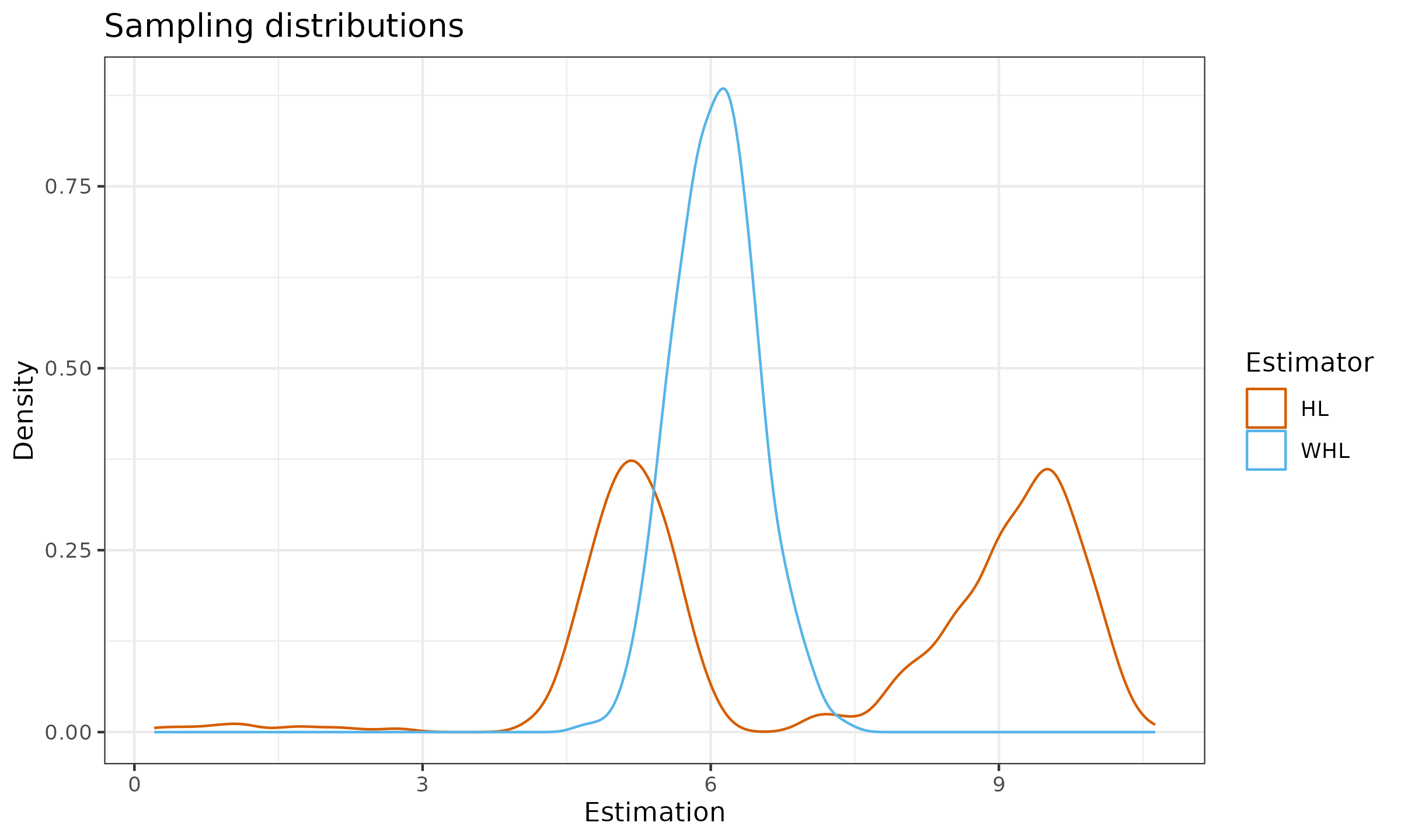
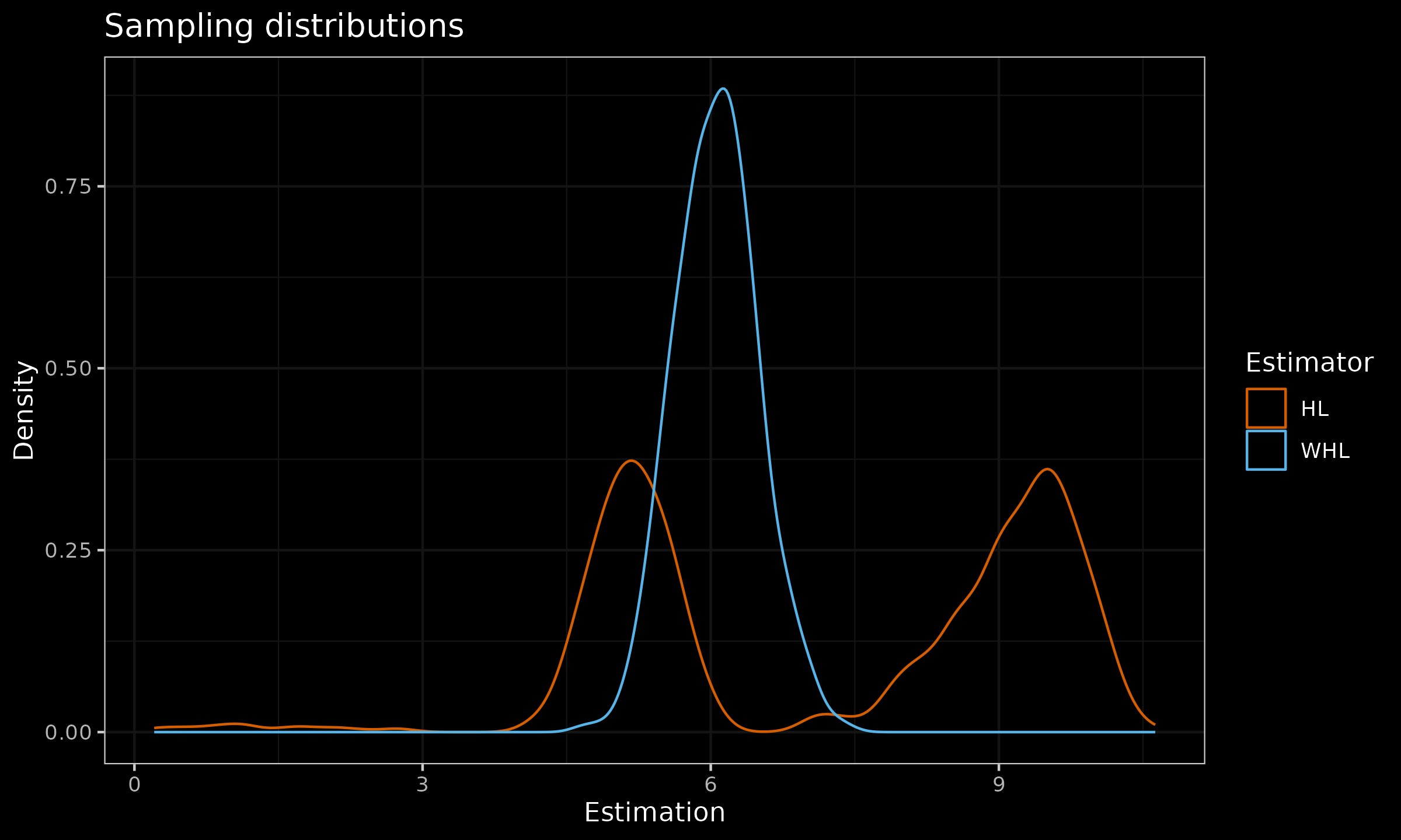
As we can see, the rebalancing of observed sub-samples from existing modes led to higher statistical efficiency and the lack of bimodality.