Winsorized modification of the Harrell-Davis quantile estimator
The Harrell-Davis quantile estimator is one of my favorite quantile estimators because of its efficiency. It has a small mean square error which allows getting accurate estimations. However, it has a severe drawback: it’s not robust. Indeed, since the estimator includes all sample elements with positive weights, its breakdown point is zero.
In this post, I want to suggest modifications of the Harrell-Davis quantile estimator which increases its robustness keeping almost the same level of efficiency.
Robustness
One of the essential properties of a statistical estimator is robustness. It describes the resistance abilities of the estimator against outliers. Robustness can be expressed using the breakdown point. The breakdown point is the proportion of invalid measurements that the estimator can handle. In other words, it’s the maximum number of sample elements that we could replace by arbitrarily large values without making the estimator value also arbitrarily large. Let’s look at a few examples.
Consider sample $x = \{ 1, 2, 3, 4, 5, 6, 7 \}$. The mean value of $x$ is $4$. Imagine that we replace one of the sample elements with $\infty$. Now the sample look like this: $x = \{ 1, 2, 3, 4, 5, 6, \infty \}$. The updated mean value is also $\infty$. It’s enough to corrupt a single element in the sample to make the mean also corrupted. The breakdown point of the mean is zero. Thus, the mean is not a robust metric.
The sample median of $x = \{ 1, 2, 3, 4, 5, 6, 7 \}$ is also $4$. However, if we replace a single sample element with $\infty$ it doesn’t make the sample median value also $\infty$. In fact, we can safely replace three elements of this sample and get $x = \{ 1, 2, 3, 4, \infty, \infty, \infty \}$. The sample median is still meaningful. It could be changed to another element from the original sample, but it will not become arbitrarily large. Thereby, we can corrupt three elements from the given seven-element sample without corrupting the sample median value. The breakdown point is $3/7\approx 43\%$. Asymptotically, the breakdown point of the sample median is $0.5$ which is the maximum possible breakdown point value. Thus, the median is a robust metric.
Efficiency
Another important estimator property is efficiency. It describes the estimator accuracy.
Consider the straightforward way to calculate the sample median for a sample of size $n$:
- If $n$ is odd, the median is the middle element of the sorted sample
- If $n$ is even, the median is the arithmetic average of the two middle elements of the sorted sample
This rule gives us the median value of the sample, but it doesn’t provide an accurate estimation of the population median.
Meanwhile, there are other quantile estimators that have better accuracy.
One of my favorite options is the Harrell-Davis quantile estimator (see A new distribution-free quantile estimator
By Frank E Harrell, C E Davis
·
1982harrell1982).
Here is the estimation for $p^\textrm{th}$ quantile:
where $I_t(a, b)$ denotes the regularized incomplete beta function, $x_{(i)}$ is the $i^\textrm{th}$ order statistic. This estimator has higher efficiency than the sample median. It means that it has a smaller variance and smaller mean squared error.
However, the Harrell-Davis quantile estimator has a serious drawback: it’s not robust. Indeed, since its value is a linear combination of all order statistics, it’s enough to corrupt a single sample element to spoil the estimation. Thus, its breakdown point is zero.
So, how should we estimate the median? The sample median gives a robust but not-so-efficient estimation. The Harrell-Davis quantile estimator gives efficient but not robust estimation.
I’m going to suggest an approach that improves the robustness of the Harrell-Davis quantile estimator keeping a decent level of efficiency. But first, we should briefly discuss trimmed and winsorized means.
Trimmed and winsorized mean
The trimmed mean (or truncated mean) is an attempt to improve the mean robustness. The idea is simple: we should sort all values in the sample, drop the first k values and the last k values, and calculate the mean of the middle elements. Let’s say we have a sample with 8 elements:
$$ x = \{x_1, x_2, x_3, x_4, x_5, x_6, x_7, x_8\}. $$If we assume that $x$ is already sorted, and we want to calculated the 25% trimmed mean, we should drop the first 25% and the last 25% of the values:
$$ x_{\textrm{trimmed}} = \{x_3, x_4, x_5, x_6\}. $$Next, we should calculate the mean of the middle elements:
$$ \overline{x_{\textrm{trimmed}}} = \dfrac{x_3 + x_4 + x_5 + x_6}{4}. $$We can also consider a similar technique called winsorization. Instead of dropping extreme values, we could replace them with the minimum and maximum elements among the remaining values. Thus, if we 25% winsorize the above sample, we get
$$ x_{\textrm{winsorized}} = \{x_3, x_3, x_3, x_4, x_5, x_6, x_6, x_6\}. $$Using the winsorized sample, we could calculate the winsorized mean:
$$ \overline{x_{\textrm{winsorized}}} = \dfrac{x_3 + x_3 + x_3 + x_4 + x_5 + x_6 + x_6 + x_6}{4}. $$The breakdown point of p% trimmed mean and p% winsorized mean is p% (the proportion of dropped/replaced element on each tail). This makes these metrics more robust than the classic mean.
Winsorized Harrell-Davis quantile estimator
Let’s go back to the Harrell-Davis quantile estimator. It estimates the $p^\textrm{th}$ quantile as a weighted sum of order statistics:
$$ q_p = \sum_{i=1}^{n} W_{i} \cdot x_{(i)} $$The weights $W_i$ can be calculated as segment areas of Beta distribution density plot with $a = p(n+1)$ and $b = (1-p)(n+1)$. For example, $n = 10, p = 0.5$ (estimating the median for 10-elements sample) gives the following plot:
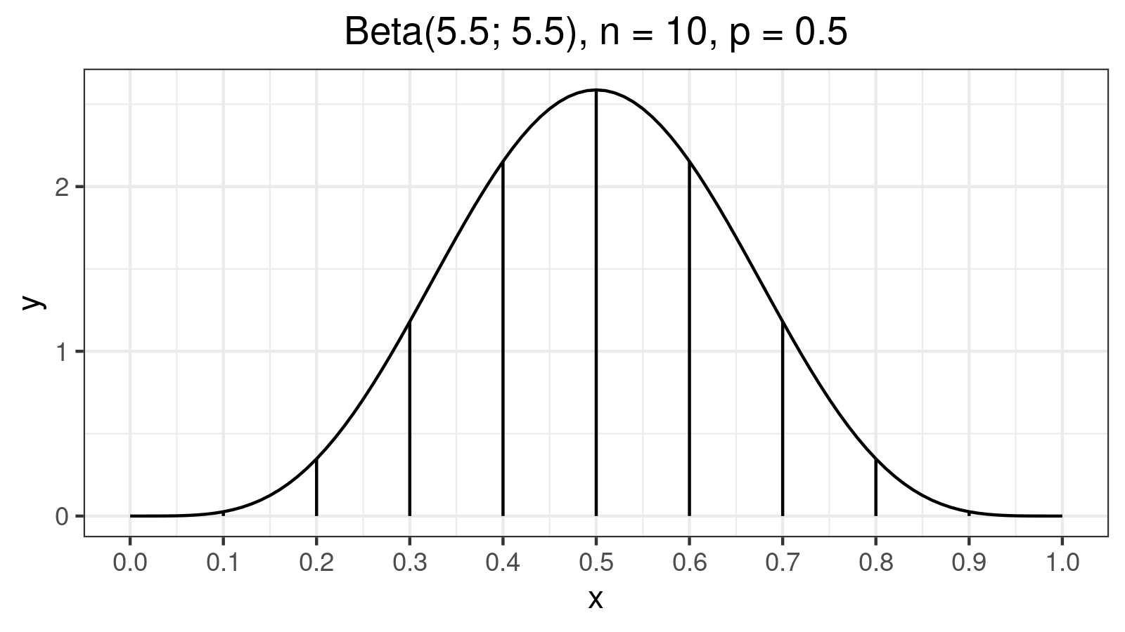

Here are the values of corresponding weights $W_i$:
W[1] = W[10] = 0.0005124147
W[2] = W[9]  = 0.0145729829
W[3] = W[8]  = 0.0727403902
W[4] = W[7]  = 0.1683691116
W[5] = W[6]  = 0.2438051006
As we can see, weights of $x_{(1)}$ and $x_{(10)}$ are $W_1 = W_{10} = 0.0005124147$. In most cases, they don’t produce a noticeable impact on the result (their total weight is about $0.1\%$). However, in the case of extremely large outliers, they can completely distort the final estimation. Let’s consider the following sample:
$$ x = \{ 1, 2, 3, 4, 5, 6, 7, 8, 9, 10 \} $$The sample median is $5.5$. The Harrell-Davis quantile estimator dives the same estimation: $q_{0.5} = 5.5$. Now let’s replace the last element of this sample by $10^6$:
$$ x = \{ 1, 2, 3, 4, 5, 6, 7, 8, 9, 10^6 \} $$Now, the Harrell-Davis estimation is $q_{0.5} = 517.9096$ which is probably too far from the actual median value. We have this problem because the Harrell-Davis quantile estimator is not robust; its breakdown point is zero.
Let’s look again at the tail elements $x_{(1)}$ and $x_{(10)}$. They are almost useless in situations without outliers and they are destructive in situations with outliers. What the point of using these values at all? What if we winsorize them?
However, we couldn’t just update the p% of values in each tail. Firstly, if we winsorize values with the big weight, we noticeably reduce the estimator efficiency. Secondly, if we estimate arbitrary quantile (not the median), the tail values may have the highest weight and definitely should not be dropped.
I suggest a simple heuristic. We should find the 99% highest density interval of the considered beta distribution. All segments outside this interval should be winsorized. Thus, we keep values that form 99% of the final result (keeping almost the same level of efficiency) and protect ourselves against outliers (improving robustness). In the below table, you can find values of breakdown points and the numbers of winsorized elements for different sample sizes.
| n | winsorized | breakdown |
|---|---|---|
| 2 | 0 | 0.0000 |
| 3 | 0 | 0.0000 |
| 4 | 0 | 0.0000 |
| 5 | 0 | 0.0000 |
| 6 | 0 | 0.0000 |
| 7 | 0 | 0.0000 |
| 8 | 2 | 0.1250 |
| 9 | 2 | 0.1111 |
| 10 | 2 | 0.1000 |
| 11 | 2 | 0.0909 |
| 12 | 4 | 0.1667 |
| 13 | 4 | 0.1538 |
| 14 | 4 | 0.1429 |
| 15 | 6 | 0.2000 |
| 16 | 6 | 0.1875 |
| 17 | 6 | 0.1765 |
| 18 | 8 | 0.2222 |
| 19 | 8 | 0.2105 |
| 20 | 8 | 0.2000 |
| 21 | 10 | 0.2381 |
| 22 | 10 | 0.2273 |
| 23 | 10 | 0.2174 |
| 24 | 12 | 0.2500 |
| 25 | 12 | 0.2400 |
| 26 | 12 | 0.2308 |
| 27 | 14 | 0.2593 |
| 28 | 14 | 0.2500 |
| 29 | 14 | 0.2414 |
| 30 | 16 | 0.2667 |
| 31 | 16 | 0.2581 |
| 32 | 18 | 0.2812 |
| 33 | 18 | 0.2727 |
| 34 | 18 | 0.2647 |
| 35 | 20 | 0.2857 |
| 36 | 20 | 0.2778 |
| 37 | 22 | 0.2973 |
| 38 | 22 | 0.2895 |
| 39 | 22 | 0.2821 |
| 40 | 24 | 0.3000 |
| 41 | 24 | 0.2927 |
| 42 | 26 | 0.3095 |
| 43 | 26 | 0.3023 |
| 44 | 26 | 0.2955 |
| 45 | 28 | 0.3111 |
| 46 | 28 | 0.3043 |
| 47 | 30 | 0.3191 |
| 48 | 30 | 0.3125 |
| 49 | 30 | 0.3061 |
| 50 | 32 | 0.3200 |
| 100 | 74 | 0.3700 |
| 500 | 442 | 0.4420 |
| 1000 | 918 | 0.4590 |
| 10000 | 9742 | 0.4871 |
| 100000 | 99184 | 0.4959 |
Winsorized Maritz-Jarrett method
The Maritz-Jarrett method (see [Maritz1979]) allows estimating quantile confidence intervals. It works great with the Harrell-Davis quantile estimator because it reuses weights $W_i$. Let’s define $k^\textrm{th}$ moment of the $p^\textrm{th}$ quantile as follows:
$$ C_k = \sum_{i=1}^n W_{i} \cdot x_{(i)}^k. $$Next, we could express the standard error of the $p^\textrm{th}$ quantile via the first and the seconds moments:
$$ s_{q_p} = \sqrt{C_2 - C_1^2} $$It’s easy to see that winsorization could be applied here as well.
Reference implementation
The C# reference implementation can be found in
the latest nightly version (0.3.0-nightly.89+) of Perfolizer
(you need WinsorizedHarrellDavisQuantileEstimator).
Conclusion
The winsorized modifications of the Harrell-Davis quantile estimator has the same level of efficiency as the original estimator, but it’s more robust. It protects the estimated value from extreme outliers. The asymptotic breakdown point of the suggested estimator is $0.5$. Also, the winsorized version can be calculated much faster because it doesn’t require so many values of the regularized incomplete beta function.
References
- [Harrell1982]
Harrell, F.E. and Davis, C.E., 1982. A new distribution-free quantile estimator. Biometrika, 69(3), pp.635-640.
https://doi.org/10.2307/2335999 - [Maritz1979]
Maritz, J. S., and R. G. Jarrett. 1978. “A Note on Estimating the Variance of the Sample Median.” Journal of the American Statistical Association 73 (361): 194–196.
https://doi.org/10.1080/01621459.1978.10480027