Weighted Mann-Whitney U test, Part 2
Previously, I suggested a weighted version of the Mann–Whitney $U$ test. The distribution of the weighted normalized $U_\circ^\star$ can be obtained via bootstrap. However, it is always nice if we can come up with an exact solution for the statistic distribution or at least provide reasonable approximations. In this post, we start exploring this distribution.
When I started my first attempts to build an approximation for the $U_\circ^\star$ distribution, I assumed that it should be asymptotically normal. Indeed, the non-weighted Mann–Whitney $U$ statistic gives us an asymptotically normal distribution with mean $nm/2$ and standard deviation $\sqrt{nm(n+m+1)/12}$. The precision of this approximation is not always good enough, but it can be improved using the Edgeworth expansion or the Saddlepoint approximation. It is tempting to assume that the weighted version should also be asymptotically normal. Since the $U_\circ^\star$ is a normalized statistic on $[0; 1]$, the mean value is obviously $0.5$. So, I spent some time trying to derive the standard deviation. These attempts were not particularly successful. Eventually, I found an example that shows that this distribution can be far from normal. This will be a short post in which I only present an example that demonstrates this non-normal behavior.
We consider two samples of equal size $n$:
$$ \mathbf{x} = ( x_1, x_2, \ldots, x_n ), \quad \mathbf{y} = ( y_1, y_2, \ldots, y_n ). $$The samples are generated according to the following rules:
$$ x_1, y_{1..n-1} \sim \mathcal{N}(10, 1), $$$$ x_{2..n}, y_n \sim \mathcal{N}(20, 1). $$We also define the following weight vectors:
$$ \mathbf{w} = ( w_1, w_2, \ldots, w_n ), \quad \mathbf{v} = ( v_1, v_2, \ldots, v_n ), $$where
$$ w_1 = 0.5,\quad w_2 = w_3 = \ldots = w_n = 0.5 / (n - 1), $$$$ v_1 = v_2 = \ldots = v_{n - 1} = 0.5 / (n - 1),\quad v_n = 0.5. $$Essentially, such configuration corresponds to a mixture of two normal distributions: $0.5 \mathcal{N}(10, 1) + 0.5 \mathcal{N}(20, 1)$. Sample $\mathbf{x}$ has one value from the first mode and $n-1$ values from the second mode. Sample $\mathbf{y}$ has $n-1$ values from the first mode and one value from the second mode. The weight vectors $\mathbf{w}$ and $\mathbf{v}$ specify the rebalancing procedure so that pairs $\langle \mathbf{x}, \mathbf{w}\rangle$ and $\langle\mathbf{y}, \mathbf{v}\rangle$ are equivalent from the weighted sampling point of view.
Now let us build the distribution of $U_\circ^\star(\mathbf{x}, \mathbf{y}, \mathbf{w}, \mathbf{v})$. Here are the corresponding density plots for $n \in \{ 10, 25, 100, 500 \}$:
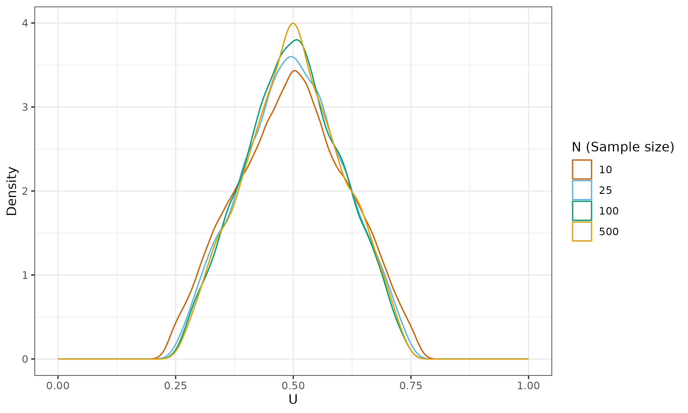
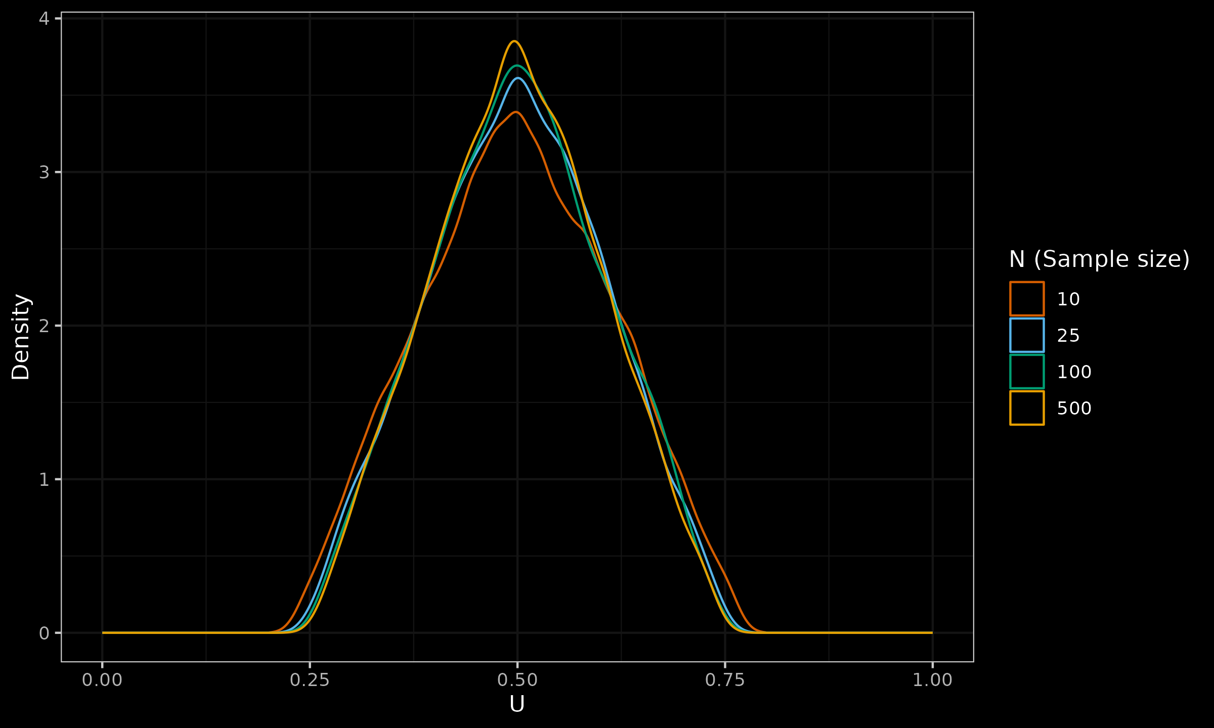
As we can see, the obtained distributions are far from normal and closer to a triangular distribution. At the moment, I do not have strict proof of non-normality for this case (theoretically, it still can converge to $\mathcal{N}(0.5, \sigma^2)$ for extremely large $n$). However, numerical simulations show that we cannot define a normal distribution that is an acceptable approximation for practical case studies.