Weighted Mann-Whitney U test, Part 3
I continue building a weighted version of the Mann–Whitney $U$ test. While previously suggested approach feel promising, I don’t like the usage of Bootstrap to obtain the $p$-value. It is always better to have a deterministic and exact approach where it’s possible. I still don’t know how to solve it in general case, but it seems that I’ve obtained a reasonable solution for some specific cases. The current version of the approach still has issues and requires additional correction factors in some cases and additional improvements. However, it passes my minimal requirements, so it is worth trying to continue developing this idea. In this post, I share the description of the weighted approach and provide numerical examples.
Classic Mann–Whitney $U$ test
We consider the one-sided Mann-Whitney U test that compares two samples $\mathbf{x}$ and $\mathbf{y}$:
$$ \mathbf{x} = ( x_1, x_2, \ldots, x_n ), \quad \mathbf{y} = ( y_1, y_2, \ldots, y_m ). $$The $U$ statistic for this test is defined as follows:
$$ U(x, y) = \sum_{i=1}^n \sum_{j=1}^m S(x_i, y_j),\quad S(a,b) = \begin{cases} 1, & \text{if } a > b, \\ 0.5, & \text{if } a = b, \\ 0, & \text{if } a < b. \end{cases} $$The $p$-value is obtained based on the distribution of the $U$ statistic. First, we discuss the non-weighted case, and only then continue with the fast implementation.
Weighted Mann–Whitney $U$ test
For the weighted version of the test, we assign vectors of weights $\mathbf{w}$ and $\mathbf{v}$ for $\mathbf{x}$ and $\mathbf{y}$ respectively.
$$ \mathbf{w} = ( w_1, w_2, \ldots, w_n ), \quad \mathbf{v} = ( v_1, v_2, \ldots, v_m ), $$where $w_i \geq 0$, $v_j \geq 0$, $\sum w_i > 0$, $\sum v_j > 0$.
Let us consider the normalized versions of the weight vectors:
$$ \overline{\mathbf{w}} = ( \overline{w}_1, \overline{w}_2, \ldots, \overline{w}_n ), \quad \overline{\mathbf{v}} = ( \overline{v}_1, \overline{v}_2, \ldots, \overline{v}_m ), $$$$ \overline{w}_i = \frac{w_i}{\sum_{k=1}^n w_k},\quad \overline{v}_j = \frac{v_j}{\sum_{k=1}^m v_k}. $$To define the weighted versions of the sample sizes, we use Kish’s effective sample size:
$$ n^\star = \frac{\Big( \sum_{i=1}^n w_i \Big)^2}{\sum_{i=1}^n w_i^2 },\quad m^\star = \frac{\Big( \sum_{j=1}^m v_i \Big)^2}{\sum_{j=1}^m v_i^2 }. $$Let us introduce the weighted version of the $U$ statistic. I suggest using the following approach:
$$ U^\star(\mathbf{x}, \mathbf{y}, \mathbf{w}, \mathbf{v}) = n^\star m^\star \cdot \sum_{i=1}^n \sum_{j=1}^m S(x_i, y_j) \cdot \overline{w}_i \cdot \overline{v}_j. $$Essentially, we used two tricks here:
- We multiply each term $S(x_i, y_j)$ by $\overline{w}_i \cdot \overline{v}_j$ in order to acknowledge the weights similarly to the weighted Hodges-Lehmann location estimator.
- We normalize the final result by acknowledging the effective sample sizes. While the original $U$ statistic is in $[0; nm]$, the weighted version is in $[0; n^\star m^\star]$. TODO
Classic Mann–Whitney $U$ test: implementation
Now, let’s discuss the implementation. First of all, I want to share my preferences for implementing the classic version. There are two ways to estimate the $p$-value: the exact one and the approximate one.
The classic approach based on the recurrence equation $p_{n,m}(u) = p_{n-1,m}(u - m) + p_{n,m-1}(u)$ is very slow and requires $\mathcal{O}(n m)$ memory. While it’s used in almost all standard implementations of the Mann–Whitney $U$ test, it’s too inefficient in practice. Fortunately, now we the Andreas Löffler’s implementation that allows us to calculate the exact $p$-value much faster using $\mathcal{O}(u)$ memory (worst case $\mathcal{O}(nm)$). It is defined as follows:
$$ p_{n,m}(u) = \frac{1}{u} \sum_{i=0}^{u-1} p_{n,m}(i) \cdot \sigma_{n,m}(u - i), $$$$ \sigma_{n,m}(u) = \sum_{u \operatorname{mod} d} \varepsilon_d d,\quad\textrm{where}\; \varepsilon_d = \begin{cases} 1, & \textrm{where}\; 1 \leq d \leq n, \\ 0, & \textrm{else}, \\ -1, & \textrm{where}\; m+1 \leq d \leq m+n. \end{cases} $$In some cases, we can’t use the exact algorithm because it’s too computationally expensive. It corresponds to two primary cases. The first one is about large sample sizes. The limitation for the classic exact implementation is much stricter than for Löffler’s algorithm, but even Löffler’s algorithm has a reasonable maximum. The second one is about middle values of the $U$ statistic for medium sample sizes (in this case, the computation time may be high, and approximation may provide good accuracy).
The classic normal approximation is too inaccurate: it may produce errors of incredible magnitude. Fortunately, we have the Edgeworth expansion, which greatly increases the approximation accuracy.
The Edgeworth expansion extends the normal approximation approach, which based on the normal distribution $\mathcal{N}(\mu_U, \sigma_U^2)$ defined by the following parameters:
$$ \mu_U = \frac{nm}{2},\quad \sigma_U = \sqrt{\frac{nm(n+m+1)}{12}}. $$The $z$-score is calculated with the continuity correction:
$$ z = \frac{U - \mu_U \pm 0.5}{\sigma_U}, $$The $p$-value is defined as follows (assuming the Edgeworth expansion to terms of order $1/m^2$):
$$ p_{E7}(z) = \Phi(z) + e^{(3)} \varphi^{(3)}(z) + e^{(5)} \varphi^{(5)}(z) + e^{(7)} \varphi^{(7)}(z), $$where
$$ e^{(3)} = \frac{1}{4!}\left( \frac{\mu_4}{\mu_2^2} - 3 \right),\quad e^{(5)} = \frac{1}{6!}\left( \frac{\mu_6}{\mu_2^3} - 15\frac{\mu_4}{\mu_2^2} + 30 \right),\quad e^{(7)} = \frac{35}{8!}\left( \frac{\mu_4}{\mu_2^2} - 3 \right)^2, $$$$ \mu_2 = \frac{nm(n+m+1)}{12}, $$$$ \mu_4 = \frac{mn(m+n+1)}{240} \bigl( 5(m^2 n + m n^2) - 2(m^2 + n^2) + 3mn - (2m + n) \bigr), $$$$ \begin{split} \mu_6 = \frac{mn(m+n+1)}{4032} \bigl( 35m^2 n^2 (m^2 + n^2) + 70 m^3 n^3 - 42 mn (m^3 + n^3) - 14 m^2 n^2 (m + n) +\\ + 16 (m^4 + n^4) - 52 mn (m^2 + n^2) - 43 m^2 n^2 + 32 (m^3 + n^3) +\\ + 14 mn (m + n) + 8 (m^2 + n^2) + 16 mn - 8 (m + n) \bigr), \end{split} $$$$ \varphi^{(k)}(z) = -\varphi(z) H_k(z), $$$$ H_3(z) = z^3 - 3z, $$$$ H_5(z) = z^5 - 10z^3 + 15z, $$$$ H_7(z) = z^7 - 21z^5 + 105z^3 - 105z. $$The switch between the exact and approximate implementations should acknowledge the business requirements: I recommended using the approximation only if the exact implementation has insufficient performance.
The tie correction may be neglected; I recommended to avoid using the nil hypothesis, and use the minimum-effect approach with a threshold that prevents between-sample tied values.
Weighted Mann–Whitney $U$ test: implementation
It is time to build a weighted version of the previously presented implementation approach.
We start with the exact version. One may assume that we can reuse the distribution of the $U$ statistics in the non-weighted case. The obvious problem here is that the weighted sample sizes $n^\star$ and $m^\star$ and the $U$ statistic itself are not integers. As the easiest way to build a weighted version, I suggest just using the rounded values. For a small accuracy improvement, we can use a linear interpolation between values rounded up and down.
The Edgeworth expansion can be easily extended to the weighted case by replacing $n$, $m$, and $U$ with $n^\star$, $m^\star$, and $U^\star$ respectively.
Numerical simulations
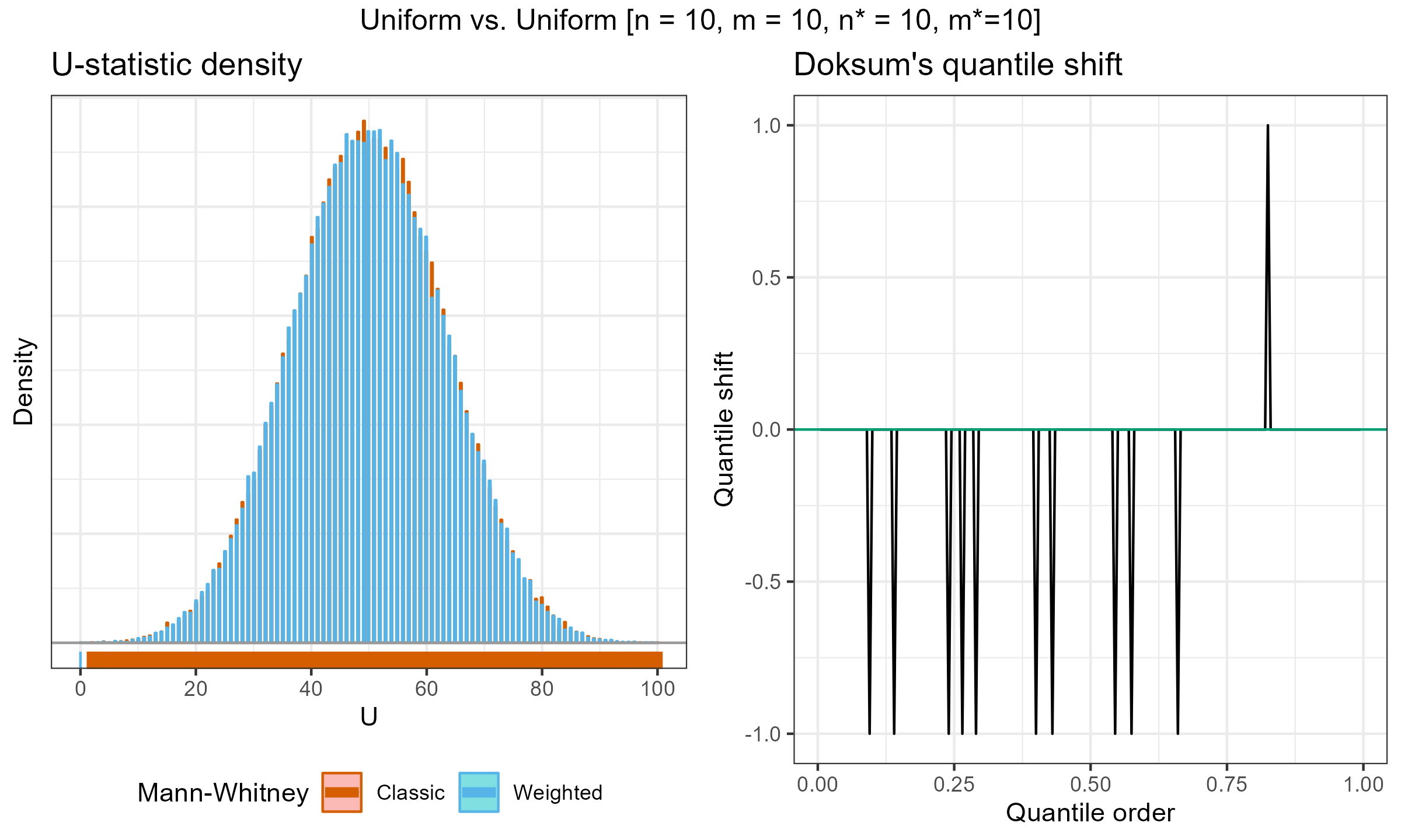
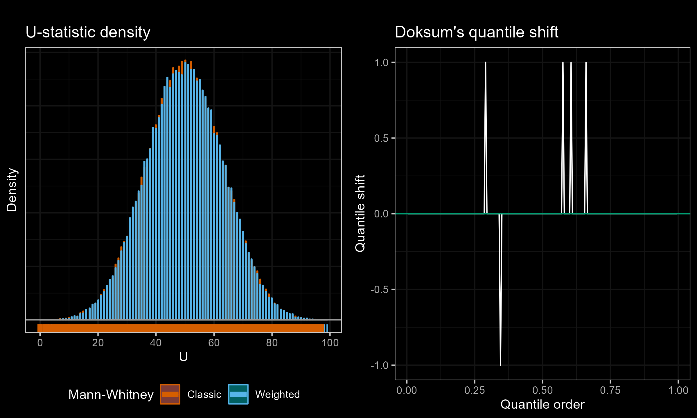
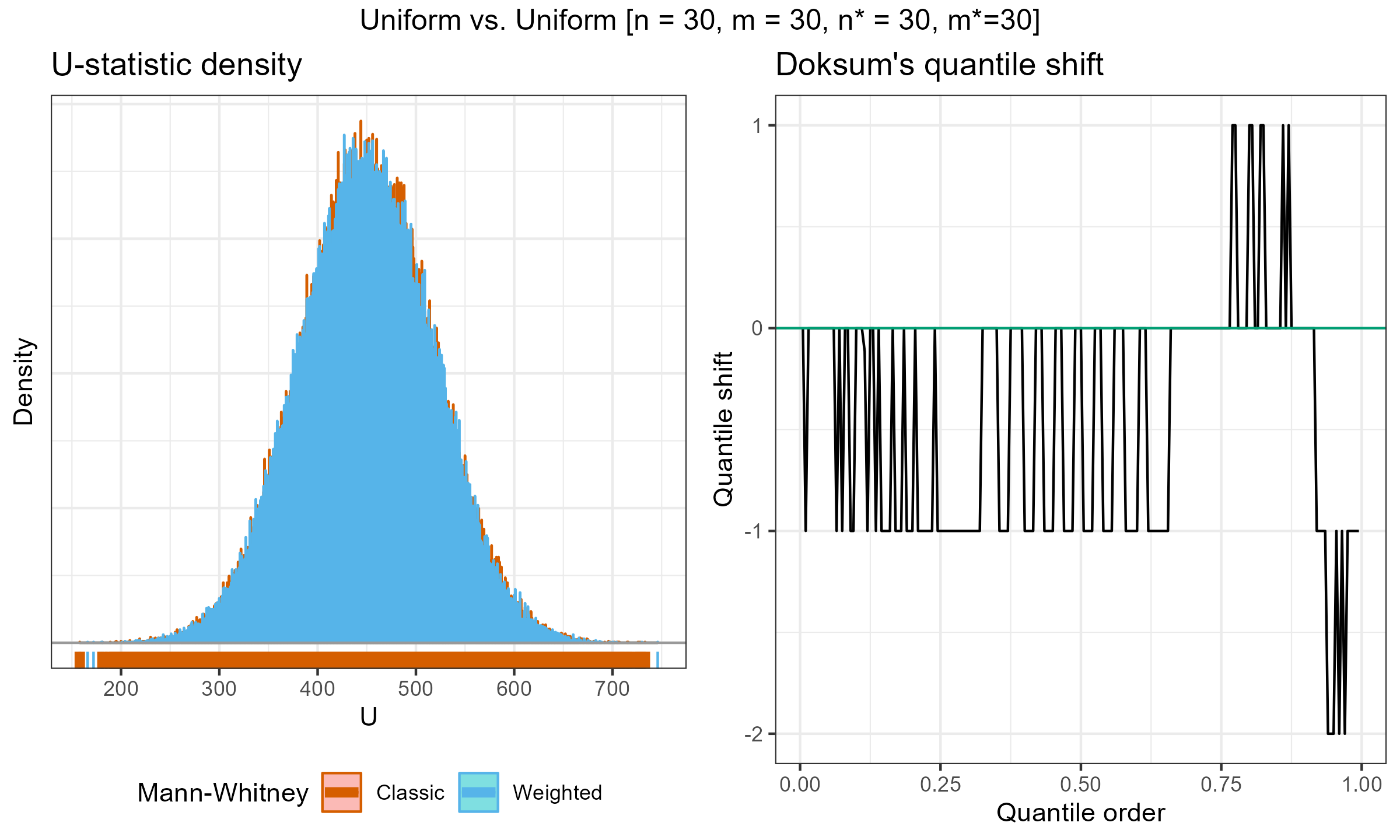
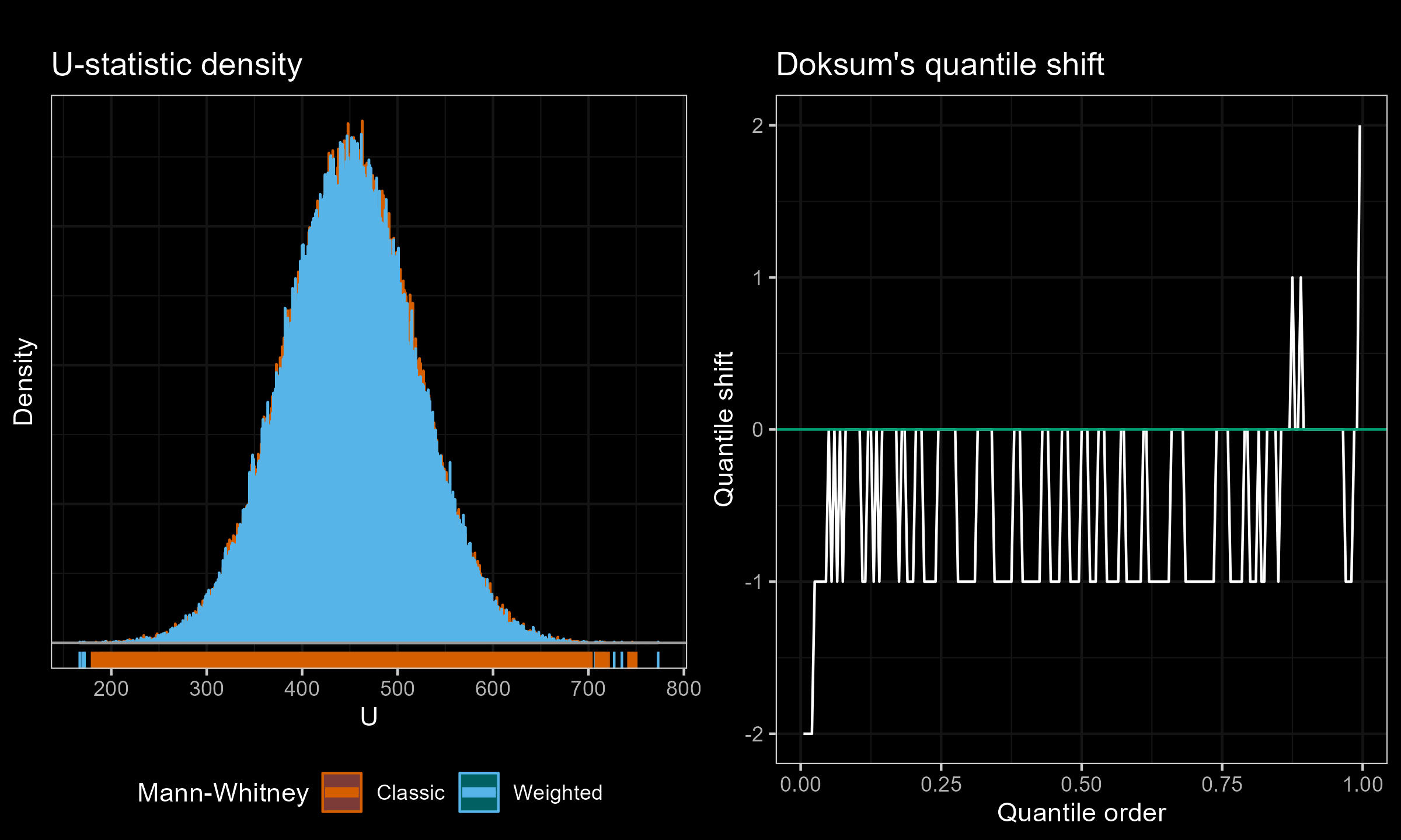
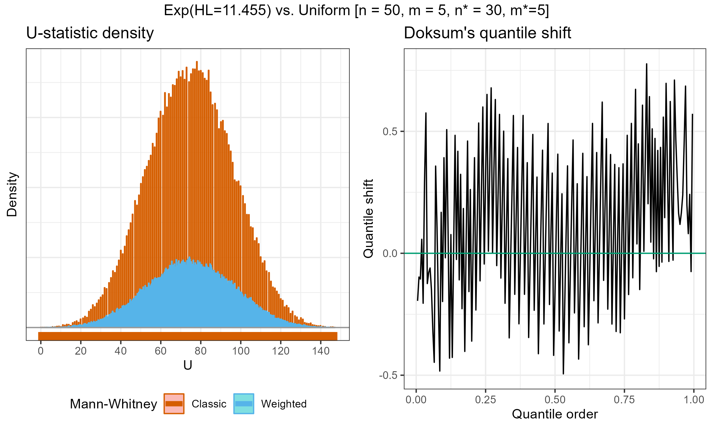
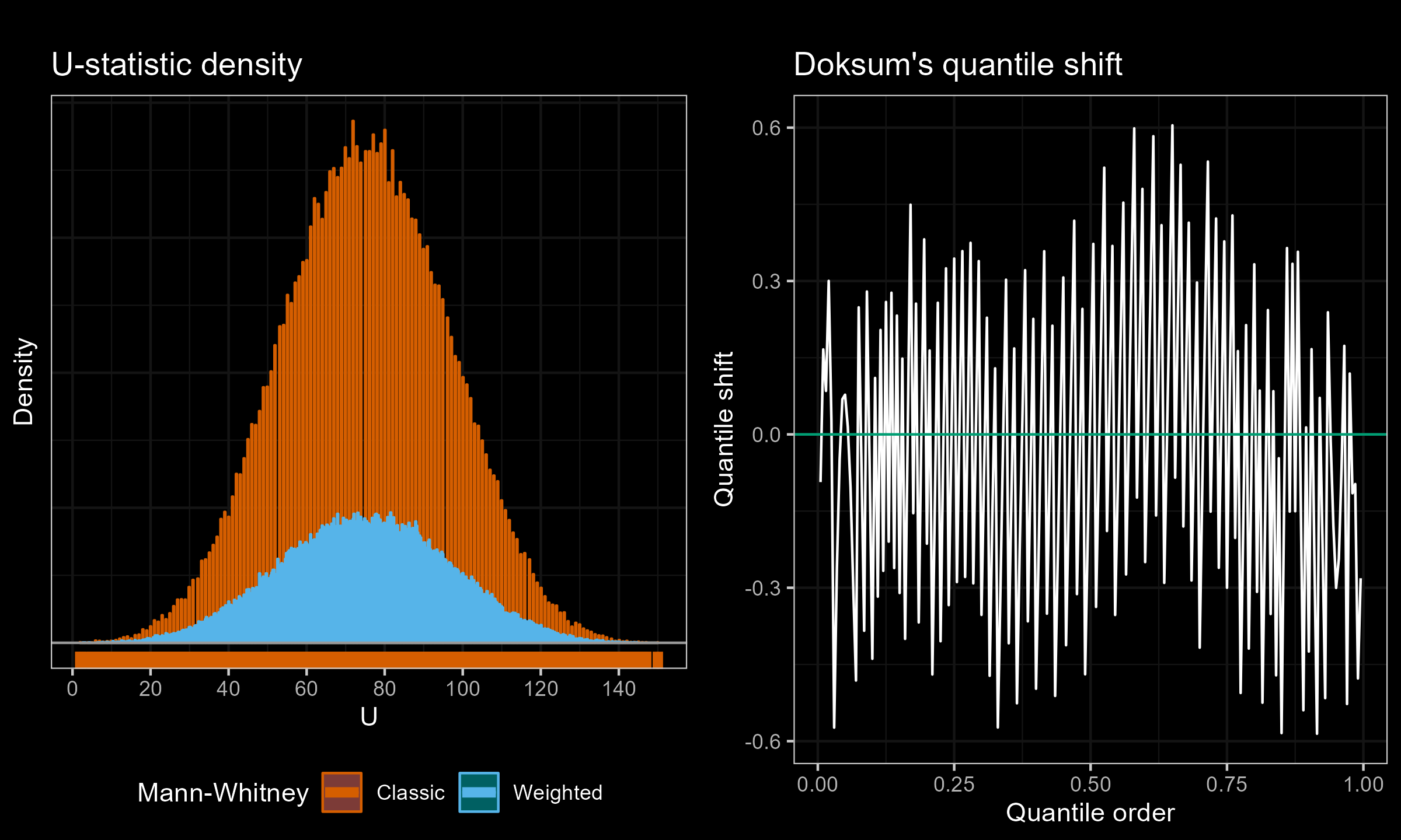
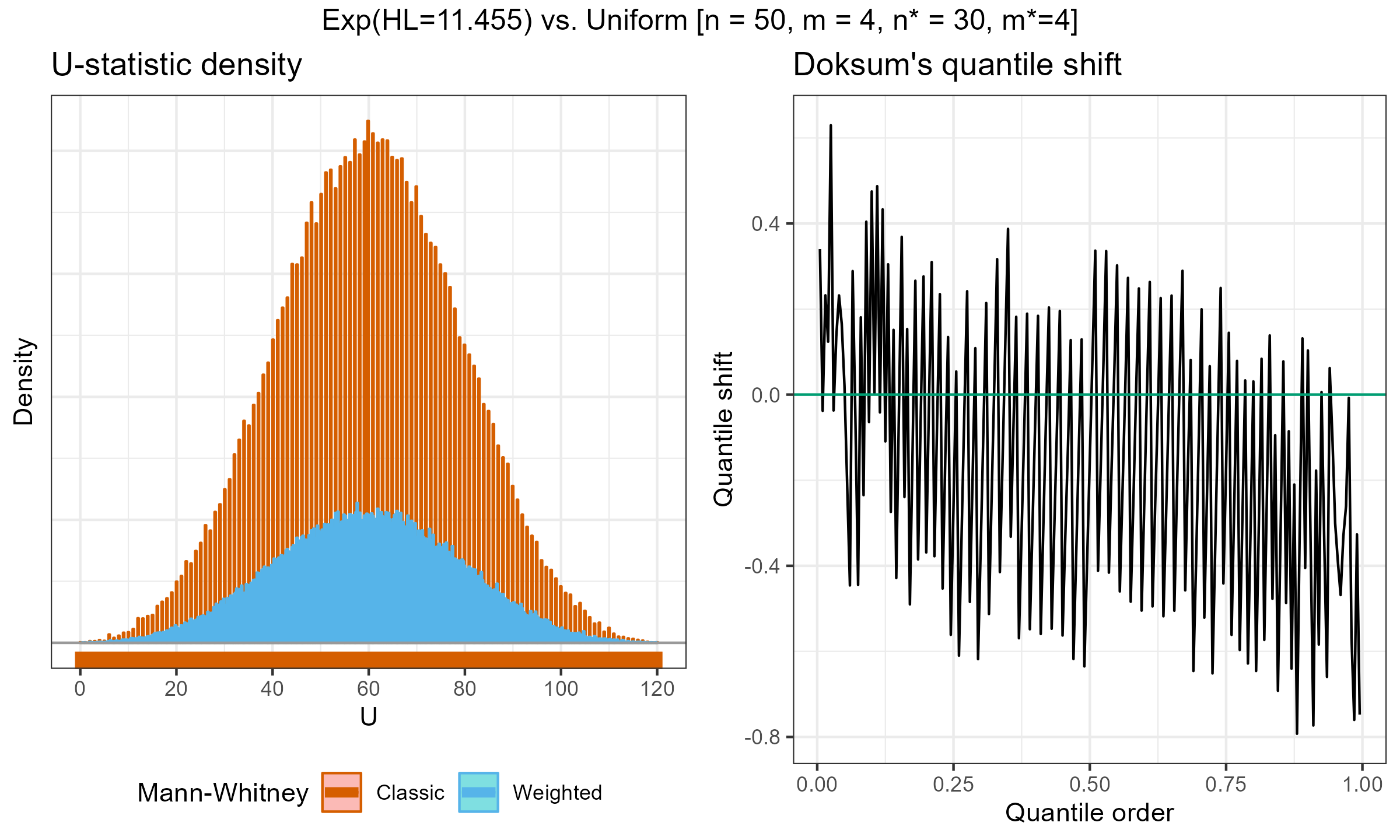
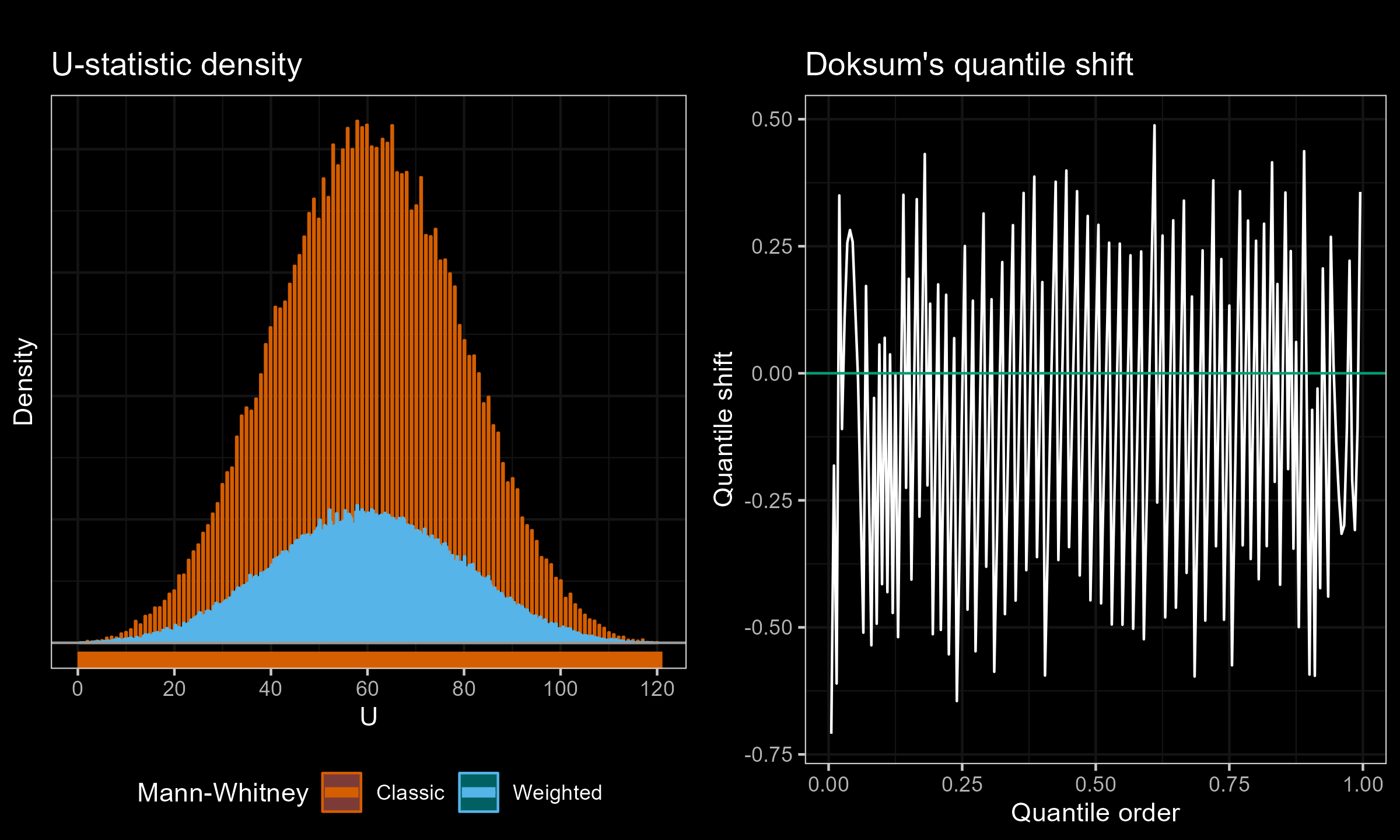
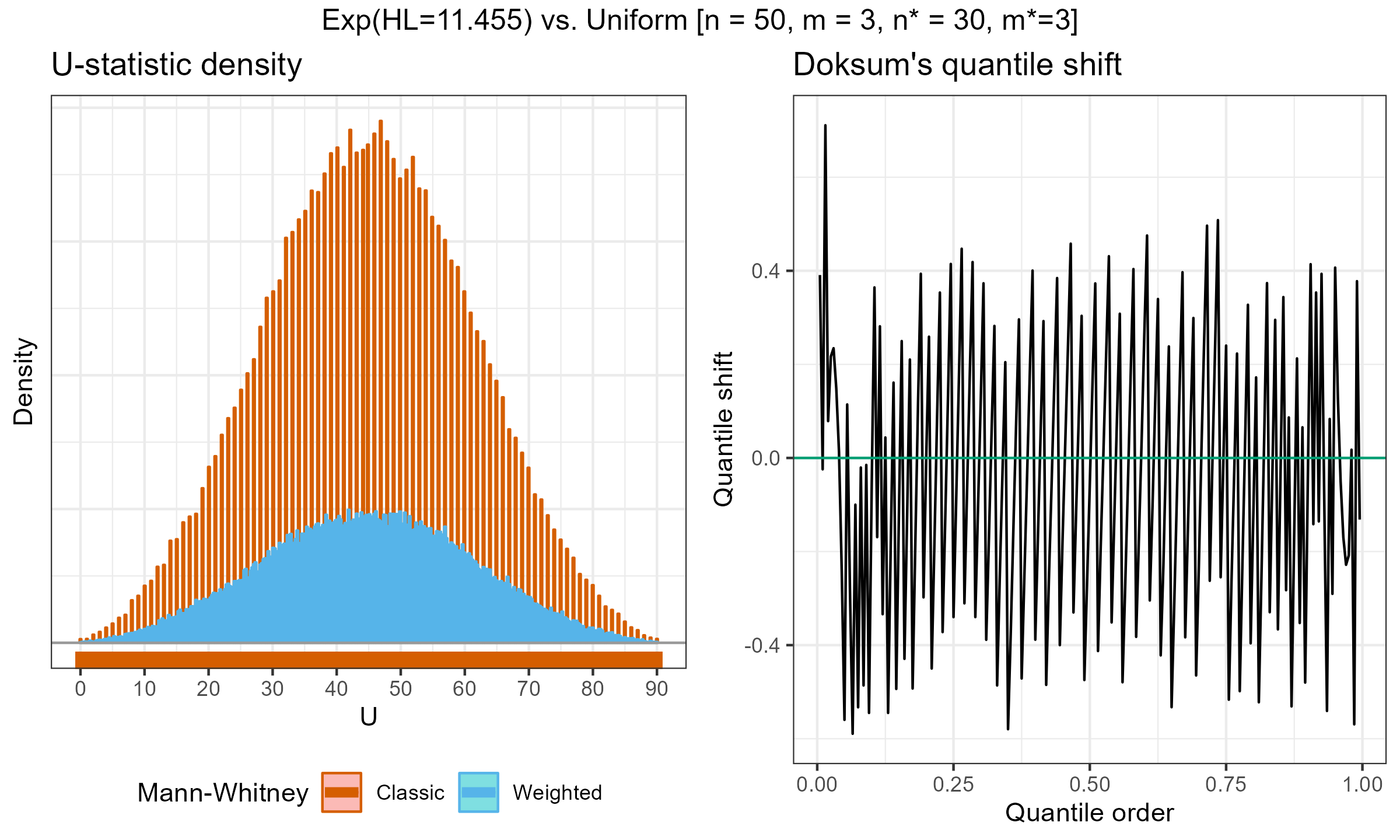
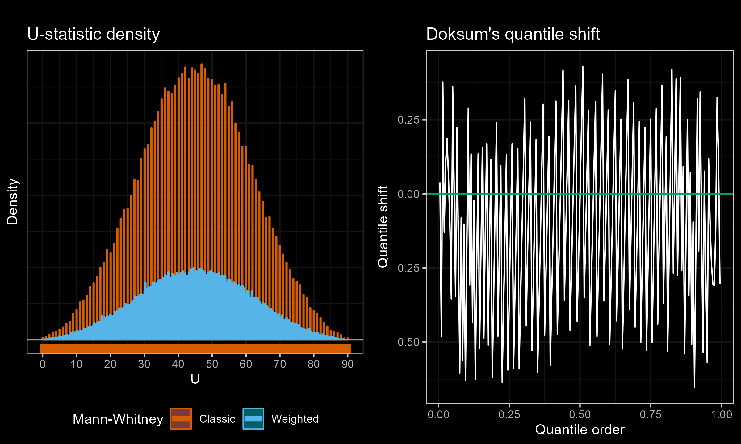
I have performed a few experiments to check how this approach works in practice. Primarily, I compared various weighted samples with uniform weighted and exponential weights parametrized by the half-life (HL). For each experiment, I’ve generated two distributions of the $U$ statistic: one using the classic Mann–Whitney $U$ test and effective sample sizes; another one using the suggested weighted approach. Next, I present density plots of these distributions, as well as Doksum’s shift quantile plots. Note that the density plot may have a different scale on the Y-axis due to the continuation process (the classic Mann–Whitney produces a discrete distribution, while the weighted version is continuous). The results of some selected experiments are presented below.
Uniform weights, $n = m = 10$:
Uniform weights, $n = m = 30$:
Exponential weights (HL=11.455) vs. Uniform weights, $n = 50$, $m = 5$:
Exponential weights (HL=11.455) vs. Uniform weights, $n = 50$, $m = 4$:
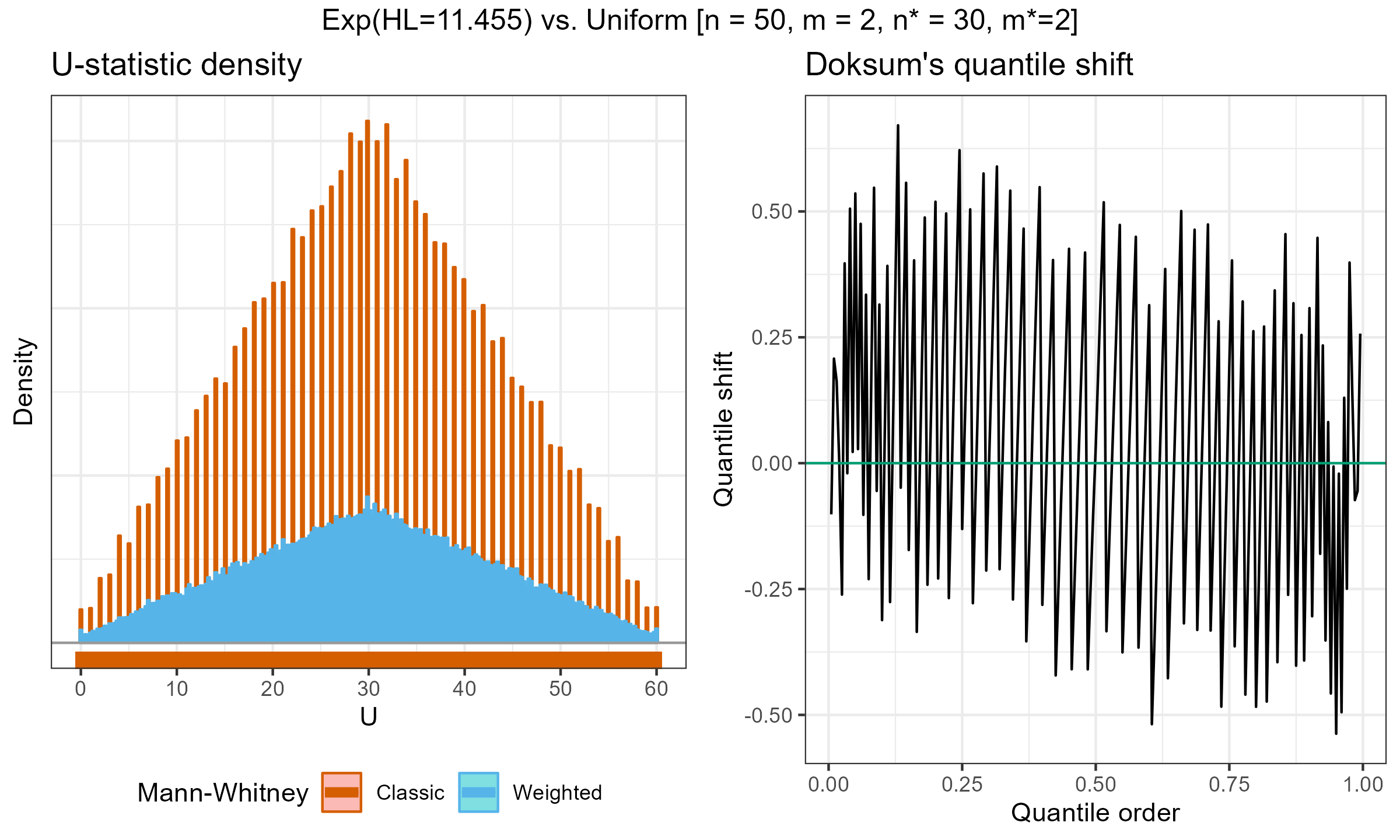
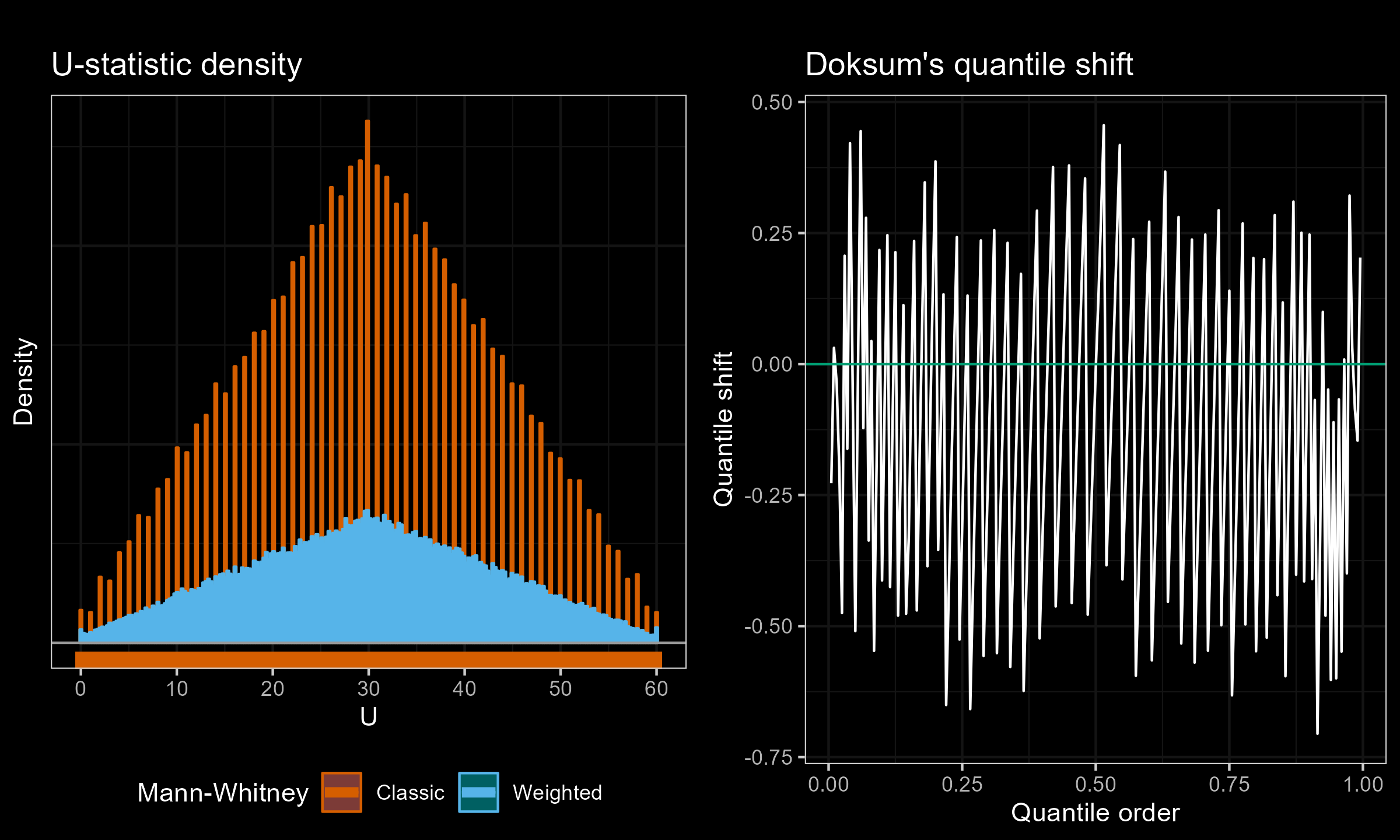
Exponential weights (HL=11.455) vs. Uniform weights, $n = 50$, $m = 2$:
Exponential weights (HL=11.455) vs. Uniform weights, $n = 50$, $m = 2$:
Exponential weights (HL=3.189) vs. Exponential weights (HL=5.154), $n=m=20$:
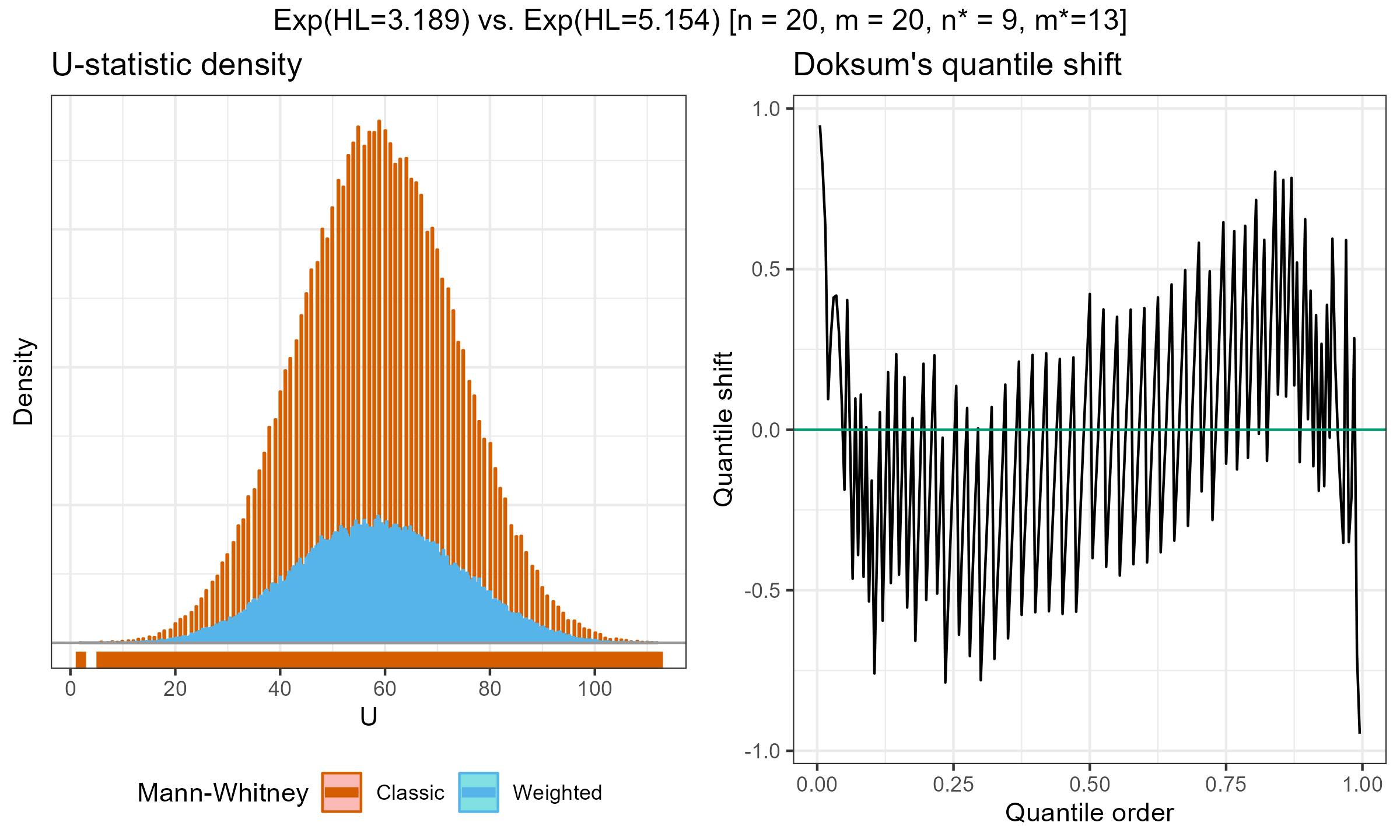
According to my observations, the approximation of the weighted version with the classic Mann–Whitney $U$-statistics distribution is quite accurate for large effective sample sizes. However, it might be inaccurate for small, effective sample sizes.
Next steps
This approach looks promising, but additional steps are required:
- Linear interpolation: we should find a proper way to handle non-integer effective sample sizes
- Small sample size correction: the suggested approach works only for reasonably large effective sample sizes; for small sample sizes, the approximation is not accurate; additional correction is needed
- Power analysis: we should check