Efficiency of the winsorized and trimmed Harrell-Davis quantile estimators

In previous posts, I suggested two modifications of the Harrell-Davis quantile estimator: winsorized and trimmed. Both modifications have a higher level of robustness in comparison to the original estimator. Also, I discussed the efficiency of the Harrell-Davis quantile estimator. In this post, I’m going to continue numerical simulation and estimate the efficiency of the winsorized and trimmed modifications.

Simulation design

The relative efficiency value depends on five parameters:

• Target quantile estimator
• Baseline quantile estimator
• Estimated quantile $p$
• Sample size $n$
• Distribution

Our target quantile estimator is the Harrell-Davis (HD) quantile estimator (harrell1982).

$$ Q_{HD}(p) = \sum_{i=1}^{n} W_{i} \cdot x_{(i)}, \quad W_{i} = I_{i/n}(a, b) - I_{(i-1)/n}(a, b), \quad a = p(n+1),\; b = (1-p)(n+1) $$

where $I_t(a, b)$ denotes the regularized incomplete beta function, $x_{(i)}$ is the $i^\textrm{th}$ order statistics. Also, we consider winsorized (WHD) and trimmed (THD) modifications of HD quantile estimator. In this simulation, we use 0.05 as the trimming percentage.

The conventional baseline quantile estimator in such simulations is the traditional quantile estimator that is defined as a linear combination of two subsequent order statistics. To be more specific, we are going to use the Type 7 quantile estimator from the Hyndman-Fan classification or HF7 (hyndman1996). It can be expressed as follows (assuming one-based indexing):

$$ Q_{HF7}(p) = x_{(\lfloor h \rfloor)}+(h-\lfloor h \rfloor)(x_{(\lfloor h \rfloor+1)})-x_{(\lfloor h \rfloor)},\quad h = (n-1)p+1. $$

Thus, we are going to estimate the relative efficiency of HD, WHD (0.05), THD (0.05) quantile estimators comparing to the traditional quantile estimator HF7. For the $p^\textrm{th}$ quantile, the relative efficiency can be calculated as the ratio of the estimator mean squared errors ($\textrm{MSE}$):

$$ \textrm{Efficiency}(p) = \dfrac{\textrm{MSE}(Q_{HF7}, p)}{\textrm{MSE}(Q_{HD}, p)} = \dfrac{\operatorname{E}[(Q_{HF7}(p) - \theta(p))^2]}{\operatorname{E}[(Q_{HD}(p) - \theta(p))^2]} $$

where $\theta(p)$ is the true value of the $p^\textrm{th}$ quantile. The $\textrm{MSE}$ value depends on the sample size $n$, so it should be calculated independently for each sample size value.

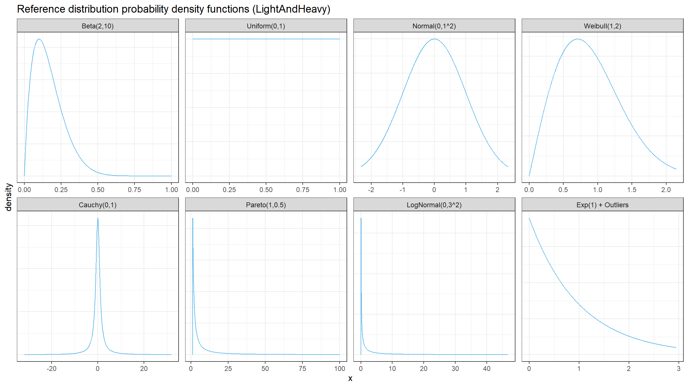
Finally, we should choose the distributions for sample generation. I decided to choose 4 light-tailed distributions and 4 heavy-tailed distributions

distribution	description
Beta(2,10)	Beta distribution with a=2, b=10
U(0,1)	Uniform distribution on [0;1]
N(0,1^2)	Normal distribution with mu=0, sigma=1
Weibull(1,2)	Weibull distribution with scale=1, shape=2
Cauchy(0,1)	Cauchy distribution with location=0, scale=1
Pareto(1, 0.5)	Pareto distribution with xm=1, alpha=0.5
LogNormal(0,3^2)	Log-normal distribution with mu=0, sigma=3
Exp(1) + Outliers	95% of exponential distribution with rate=1 and 5% of uniform distribution on [0;10000]

Here are the probability density functions of these distributions:

For each distribution, we are going to do the following:

• Enumerate all the percentiles and calculate the true percentile value $\theta(p)$ for each distribution
• Enumerate different sample sizes (from 3 to 40)
• Generate a bunch of random samples, estimate the percentile values using all estimators, calculate the relative efficiency of all target quantile estimators quantile estimator.

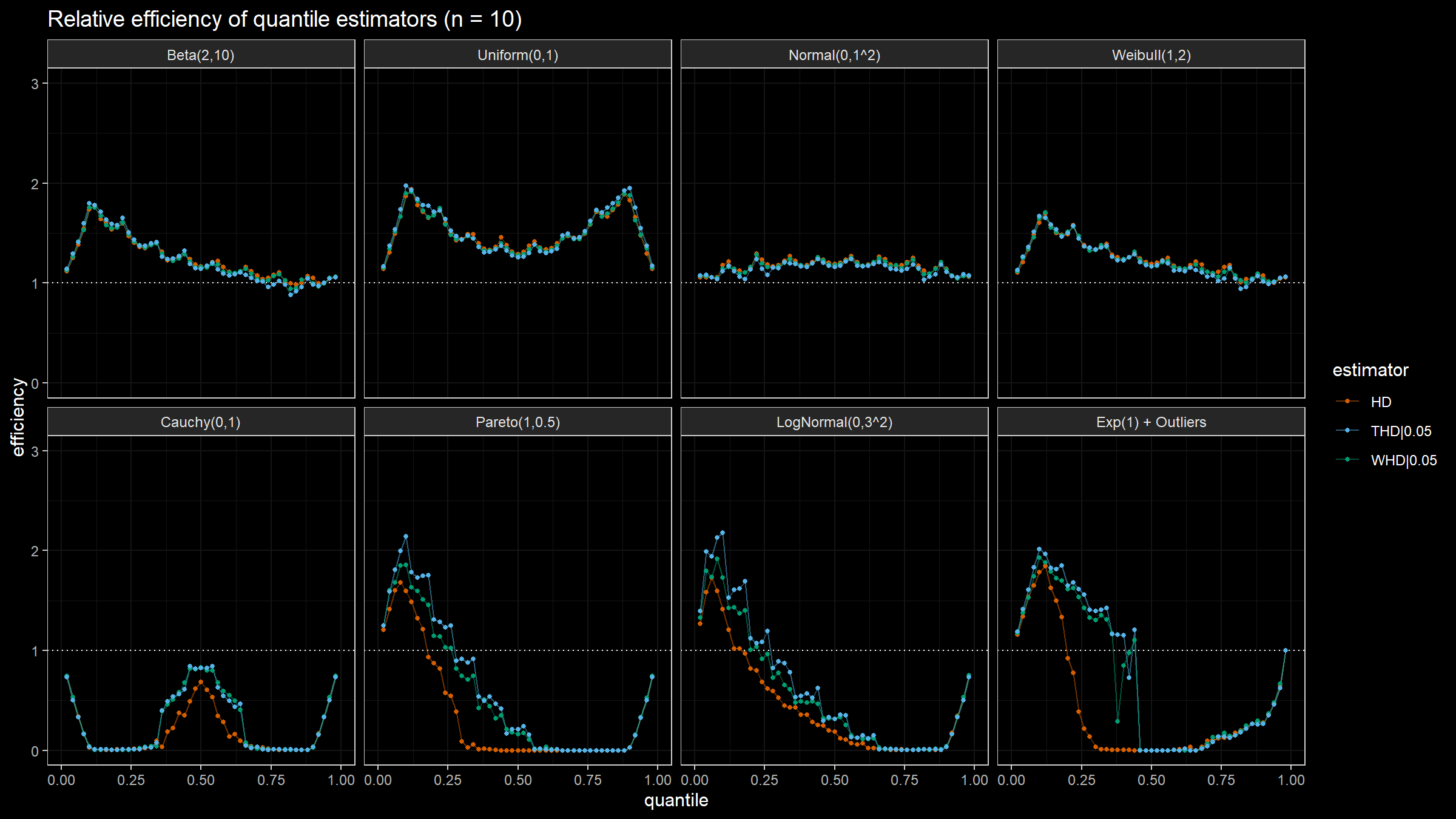
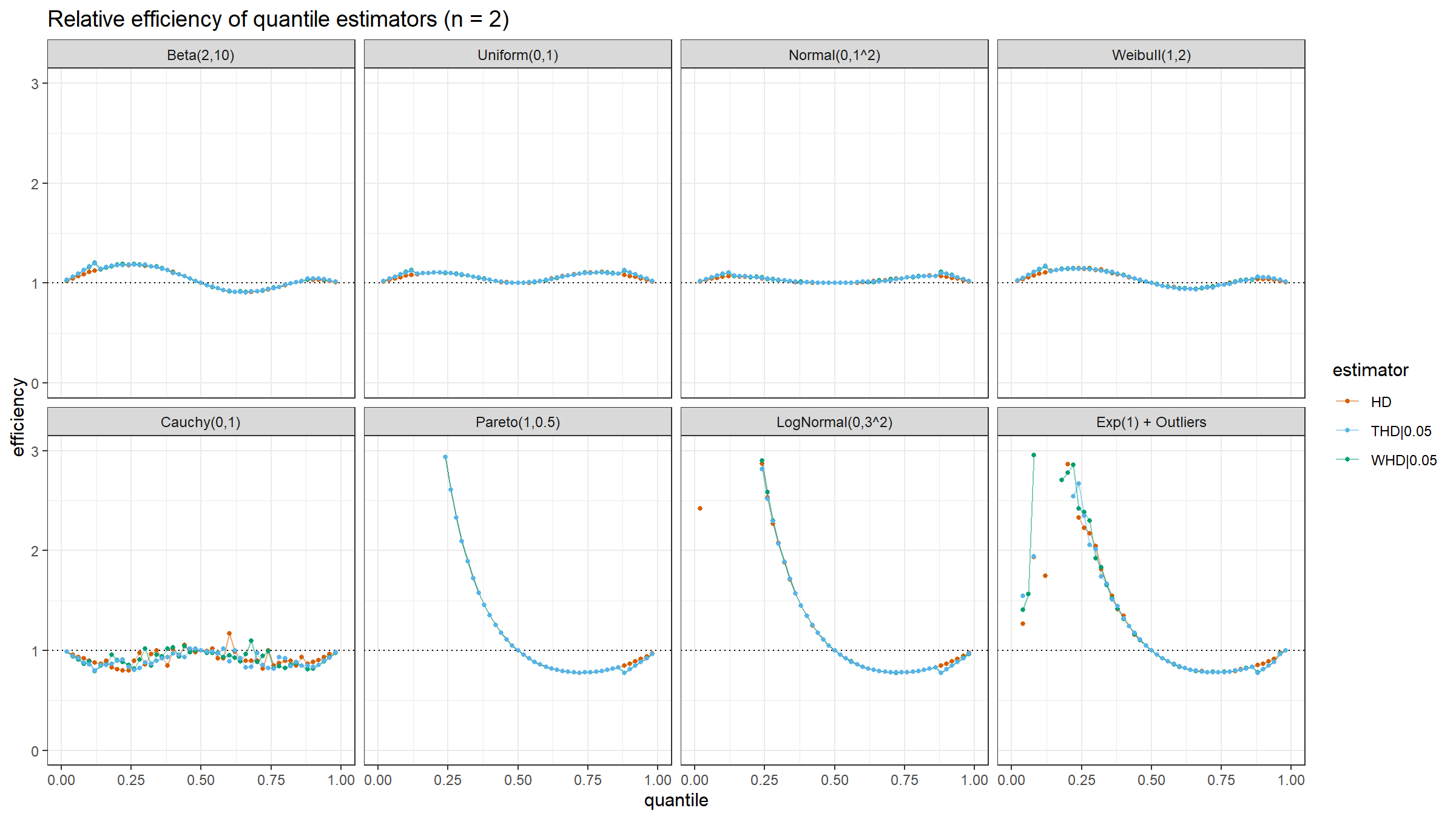
Here are the results of the simulation:

Conclusion

Based on the above simulation, we could draw the following conclusions:

• In the case of light-tailed distributions, the difference between the estimator efficiencies is insignificant.
• In the case of heavy-tailed distributions, the trimmed and winsorized modifications of the Harrell-Davis quantile estimator have higher relative efficiency values than the original estimator because they are more robust against outliers. The trimmed modification seems to be the most efficient.

References

• [Harrell1982]
  Harrell, F.E. and Davis, C.E., 1982. A new distribution-free quantile estimator. Biometrika, 69(3), pp.635-640.
  https://doi.org/10.2307/2335999
• [Hyndman1996]
  Hyndman, R. J. and Fan, Y. 1996. Sample quantiles in statistical packages, American Statistician 50, 361–365.
  https://doi.org/10.2307/2684934