Calculating gamma effect size for samples with zero median absolute deviation
In previous posts, I discussed the gamma effect size which is a Cohen’s d-consistent nonparametric and robust measure of the effect size. Also, I discussed various ways to customize this metric and adjust it to different kinds of business requirements. In this post, I want to briefly cover one more corner case that requires special adjustments. We are going to discuss the situation when the median absolute deviation is zero.
Recall
First of all, recall the general equation for the gamma effect size for the $p^\textrm{th}$ quantile:
$$ \gamma_p = \frac{Q_p(y) - Q_p(x)}{\operatorname{PMAD}_{xy}} $$where $Q_p$ is a quantile estimator of the $p^\textrm{th}$ quantile, $\operatorname{PMAD}_{xy}$ is the pooled median absolute deviation:
$$ \operatorname{PMAD}_{xy} = \sqrt{\frac{(n_x - 1) \operatorname{MAD}^2_x + (n_y - 1) \operatorname{MAD}^2_y}{n_x + n_y - 2}}, $$$\operatorname{MAD}_x$ and $\operatorname{MAD}_y$ are the median absolute deviations of $x$ and $y$:
$$ \operatorname{MAD}_x = C_{n_x} \cdot Q_{0.5}(|x_i - Q_{0.5}(x)|), \quad \operatorname{MAD}_y = C_{n_y} \cdot Q_{0.5}(|y_i - Q_{0.5}(y)|), $$$C_{n_x}$ and $C_{n_y}$ are consistency constants that makes $\operatorname{MAD}$ a consistent estimator for the standard deviation estimation.
The problem
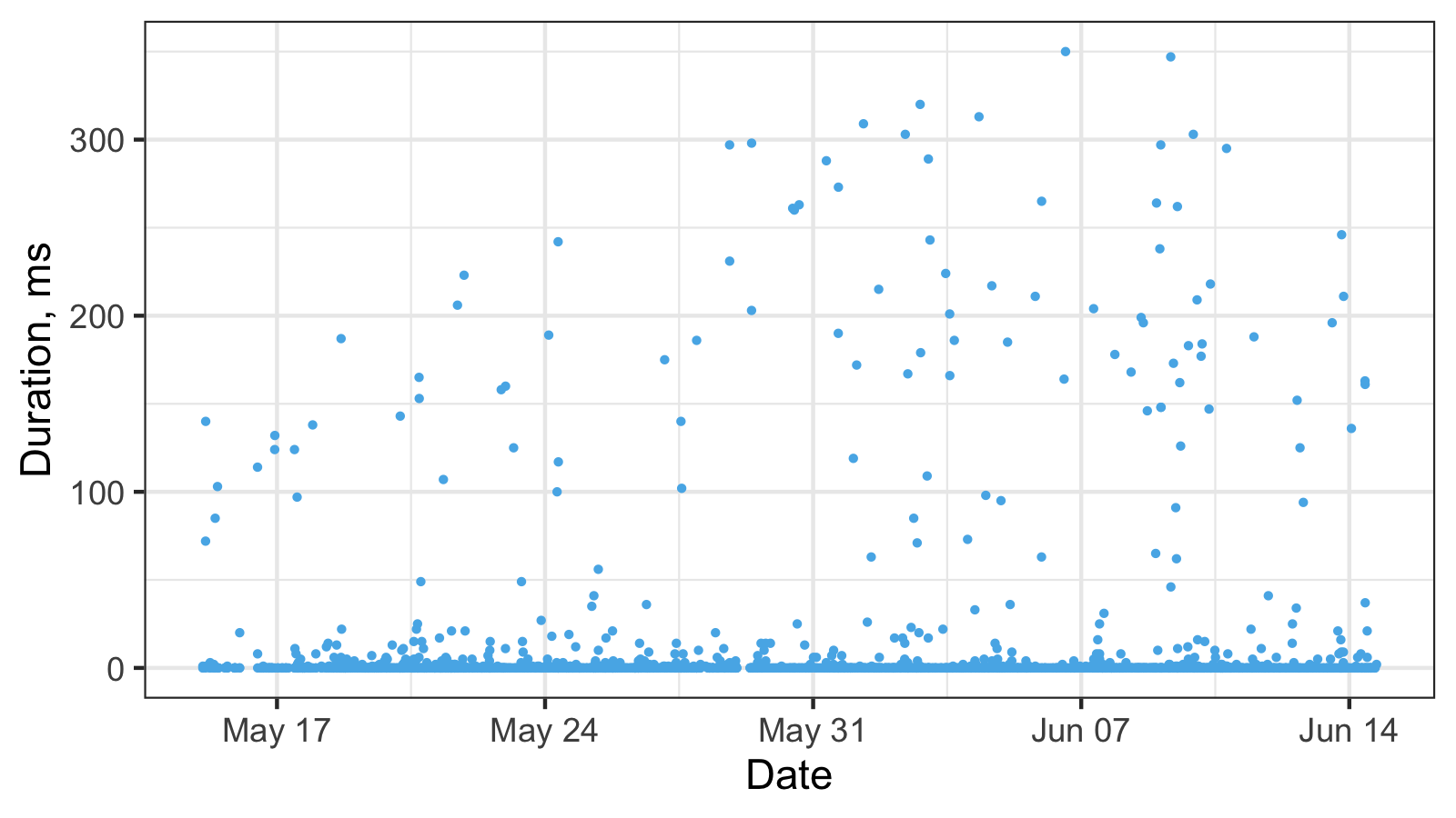
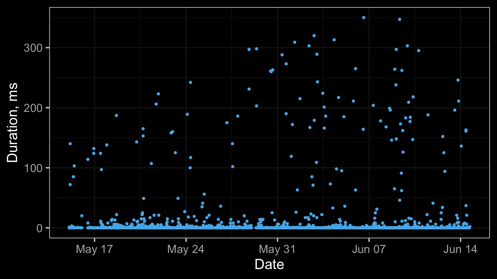
Here is a real-life dataset from my previous post:
And here is the corresponding histogram:
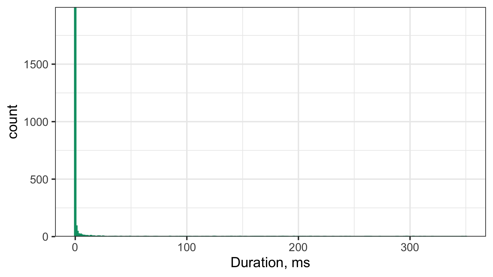
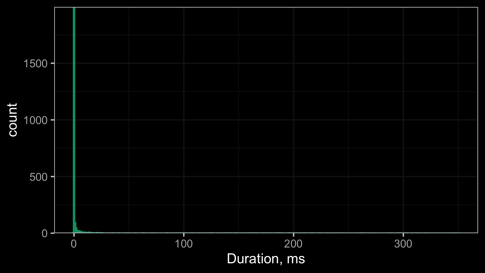
It’s hard to work with such a histogram because of the scale, so here is its raw data:
   0    1    2    3    4    5    6    7    8    9   10   11   12   13   14   15
1996   92   45   23   20   21   14    5   11    5    8    8    3    3    9    5
  16   17   18   19   20   21   22   23   25   26   27   31   33   34   35   36
   3    5    1    1    3    5    4    1    4    1    1    1    1    1    1    2
  37   41   46   49   56   62   63   65   71   72   73   85   91   94   95   97
   1    2    1    2    1    1    2    1    1    1    1    2    1    1    1    1
  98  100  102  103  107  109  114  117  119  124  125  126  132  136  138  140
   1    1    1    1    1    1    1    1    1    2    2    1    1    1    1    2
 143  146  147  148  152  153  158  160  161  162  163  164  165  166  167  168
   1    1    1    2    1    1    1    1    1    1    1    1    1    1    1    1
 172  173  175  177  178  179  183  184  185  186  187  188  189  190  196  199
   1    1    1    1    1    1    1    1    1    2    1    1    1    1    2    1
 201  203  204  206  209  211  215  217  218  223  224  231  238  242  243  246
   1    1    1    1    1    2    1    1    1    1    1    1    1    1    1    1
 260  261  262  263  264  265  273  288  289  295  297  298  303  309  313  320
   1    1    1    1    1    1    1    1    1    1    2    1    2    1    1    1
 347  350
   1    1
These numbers mean the follow: we observed 0ms 1996 times, 1ms 92 times, 2ms 45 times, and so on.
And here are the same set of numbers scaled to percents:
    0     1     2     3     4     5     6     7     8     9    10    11    12
82.68  3.81  1.86  0.95  0.83  0.87  0.58  0.21  0.46  0.21  0.33  0.33  0.12
   13    14    15    16    17    18    19    20    21    22    23    25    26
 0.12  0.37  0.21  0.12  0.21  0.04  0.04  0.12  0.21  0.17  0.04  0.17  0.04
   27    31    33    34    35    36    37    41    46    49    56    62    63
 0.04  0.04  0.04  0.04  0.04  0.08  0.04  0.08  0.04  0.08  0.04  0.04  0.08
   65    71    72    73    85    91    94    95    97    98   100   102   103
 0.04  0.04  0.04  0.04  0.08  0.04  0.04  0.04  0.04  0.04  0.04  0.04  0.04
  107   109   114   117   119   124   125   126   132   136   138   140   143
 0.04  0.04  0.04  0.04  0.04  0.08  0.08  0.04  0.04  0.04  0.04  0.08  0.04
  146   147   148   152   153   158   160   161   162   163   164   165   166
 0.04  0.04  0.08  0.04  0.04  0.04  0.04  0.04  0.04  0.04  0.04  0.04  0.04
  167   168   172   173   175   177   178   179   183   184   185   186   187
 0.04  0.04  0.04  0.04  0.04  0.04  0.04  0.04  0.04  0.04  0.04  0.08  0.04
  188   189   190   196   199   201   203   204   206   209   211   215   217
 0.04  0.04  0.04  0.08  0.04  0.04  0.04  0.04  0.04  0.04  0.08  0.04  0.04
  218   223   224   231   238   242   243   246   260   261   262   263   264
 0.04  0.04  0.04  0.04  0.04  0.04  0.04  0.04  0.04  0.04  0.04  0.04  0.04
  265   273   288   289   295   297   298   303   309   313   320   347   350
 0.04  0.04  0.04  0.04  0.04  0.08  0.04  0.08  0.04  0.04  0.04  0.04  0.04
Thus, we observed 0ms in the 92.69% cases, 1ms in the 3.81% cases, 2ms in 1.86% cases, and so on.
In this data set, both the median and the median absolute deviations are zero.
Here the observed data could be perfectly described using the
discrete Weibull distribution.
If we try to compare samples from similar distributions using the gamma effect size, we get a problem because of the zero denominator.
QAD to the rescue
In the above scenario, it’s meaningless to compare medians values. We can have a situation of different distributions with equal median values (and zero median absolute deviations). In such cases, it makes sense to compare higher quantiles instead of the median. However, it doesn’t solve the zero denominator problem.
The problem can be solved using the Quantile Absolute Deviation(QAD) around the given quantile:
$$ \operatorname{QAD}_x(p, q) = C_n \cdot Q_q(|x_i - Q_p(x)|) $$It’s easy to see that the $\operatorname{MAD}$ is just a special case of $\operatorname{QAD}$:
$$ \operatorname{MAD}_x = \operatorname{QAD}_x(0.5, 0.5). $$By analogy with $\operatorname{MAD}$, we can define the pooled quantile absolute deviation $\operatorname{PQAD}_{xy}$:
$$ \operatorname{PQAD}_{xy}(p, q) = \sqrt{\frac{ (n_x - 1) \operatorname{QAD}^2_x(p, q) + (n_y - 1) \operatorname{QAD}^2_y(p, q)}{n_x + n_y - 2}}, $$When we estimate the gamma effect size of the $p^\textrm{th}$ quantile $\gamma_p$, it makes perfect sense to evaluate the quantile absolute deviation around the same quantile. Although I don’t have specific recommendations for the value of $q$, we can start with $q=0.5$ as a starting point and adjust it if necessary.
Conclusion
We should always remember that real-life data contains tons of corner cases that may become a problem if we want to analyze this data. It’s better to think about these corner cases in advance and come up with proper solutions. In this post, we patched the gamma effect size for distribution with zero median absolute deviation using the quantile absolute deviation. This trick allows comparing higher quantiles for such distributions. A typical real-life example is the Weibull distribution.